Time Series From Scratch: Predicting What Comes Next

Exponential smoothing, ARIMA, and GARCH — three tools, one goal

1. The Problem: What Will Tomorrow’s Value Be?

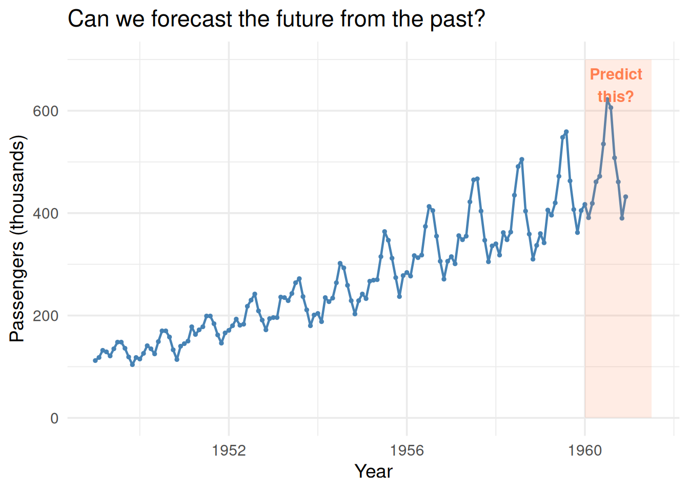
You have data ordered in time — daily sales, monthly temperatures, hourly stock prices. The past has a pattern. Can you extend that pattern into the future?

This is forecasting: using the history of a value to predict where it’s going next.

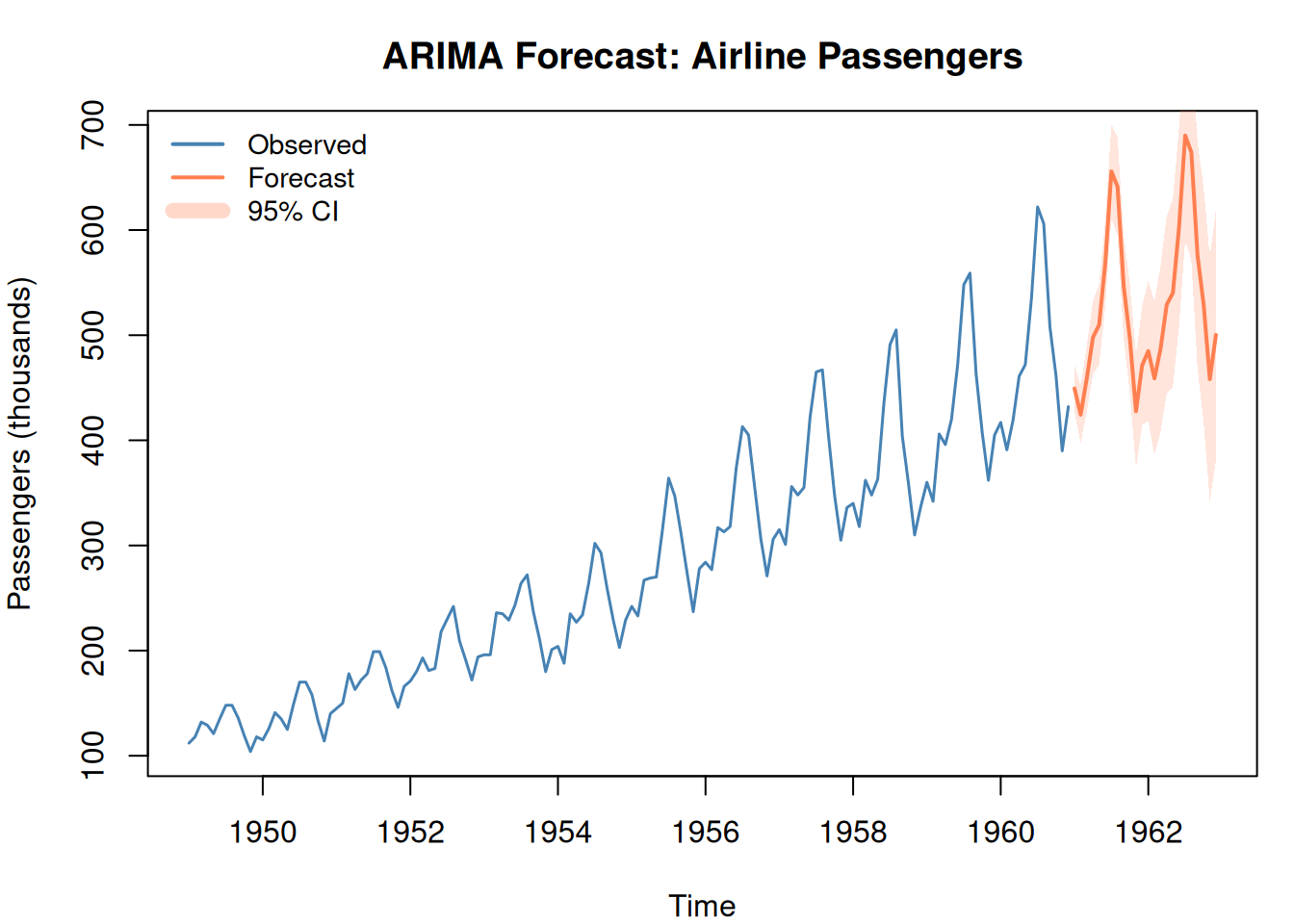
library(ggplot2)

# Classic airline passengers dataset
ap <- AirPassengers
df_ap <- data.frame(
  time = as.numeric(time(ap)),
  passengers = as.numeric(ap)
)

ggplot(df_ap, aes(time, passengers)) +
  geom_line(linewidth = 0.8, color = "steelblue") +
  geom_point(size = 0.8, color = "steelblue") +
  annotate("rect", xmin = 1960, xmax = 1961.5, ymin = 0, ymax = 700,
           fill = "coral", alpha = 0.15) +
  annotate("text", x = 1960.7, y = 650, label = "Predict\nthis?",
           color = "coral", fontface = "bold", size = 4) +
  theme_minimal(base_size = 14) +
  labs(x = "Year", y = "Passengers (thousands)",
       title = "Can we forecast the future from the past?")

Figure 1: Monthly airline passengers — a clear trend and seasonal pattern. What comes next?

Three patterns appear in time series data:

Pattern	What it looks like	Example
Level	Flat, bouncing around a constant	Daily temperature in a stable climate
Trend	Going steadily up or down	Company revenue growing year over year
Seasonality	Repeating cycle at fixed intervals	Retail sales spiking every December

Different forecasting methods handle different combinations of these.

2. Exponential Smoothing: The Weighted Average Approach

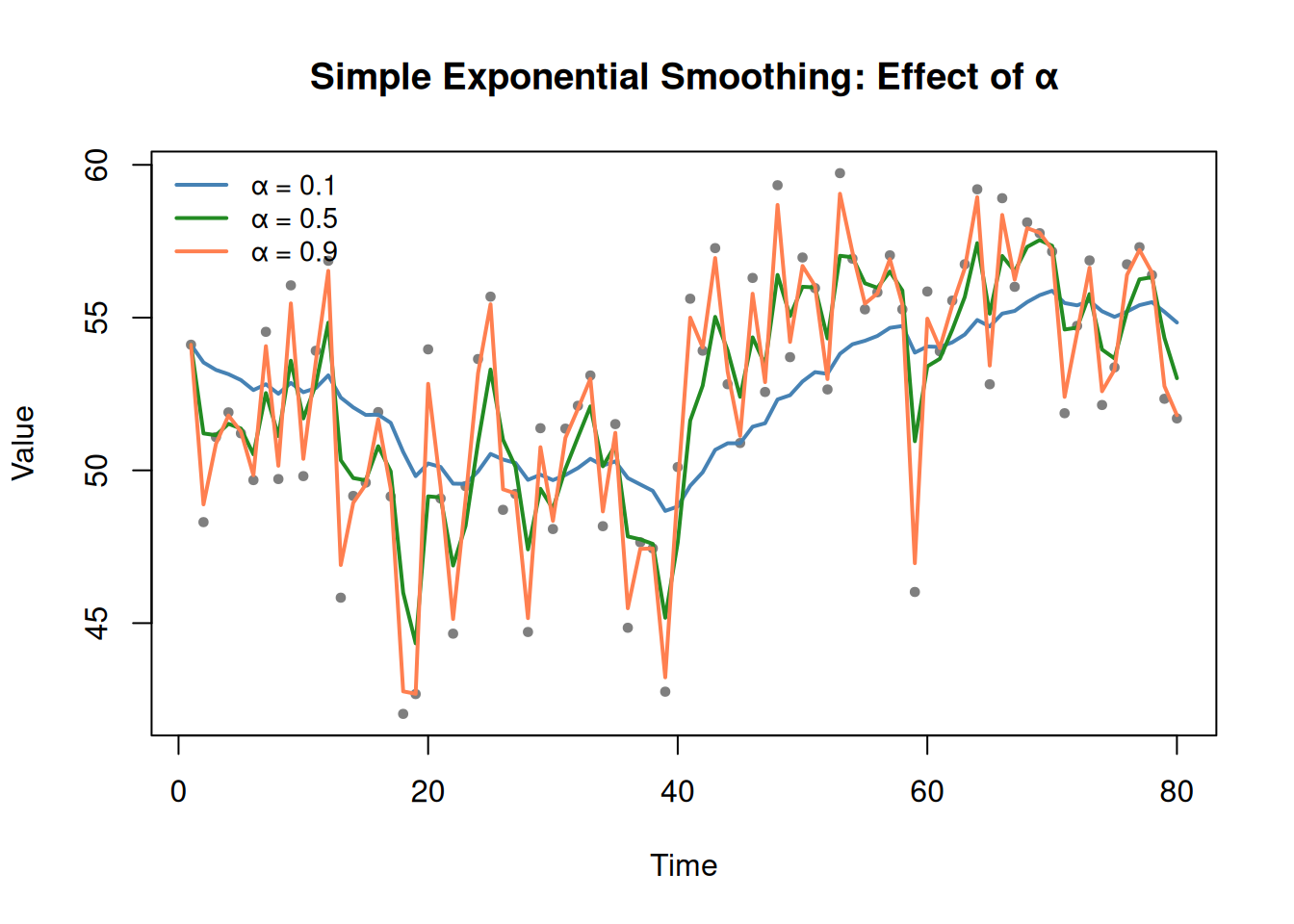
Simple Exponential Smoothing (Level Only)

The simplest idea: your forecast is a weighted average of the current observation and your previous forecast.

\[S_t = \alpha \cdot x_t + (1 - \alpha) \cdot S_{t-1}\]

\[\text{Forecast: } \hat{x}_{t+1} = S_t\]

Symbol	What it is	Plain English
\(S_t\)	Smoothed value at time \(t\)	Your best estimate of the current level
\(x_t\)	Actual observation at time \(t\)	What really happened
\(S_{t-1}\)	Previous smoothed value	What you predicted last time
\(\alpha\)	Smoothing parameter (0 to 1)	How much to trust the new data vs the old estimate
\(\hat{x}_{t+1}\)	Forecast for next period	Your prediction

The key insight: \(\alpha\) controls how much memory the model has.

• High \(\alpha\) (near 1): Mostly trusts the latest observation → reactive, follows changes quickly, but noisy
• Low \(\alpha\) (near 0): Mostly trusts the history → smooth, stable, but slow to react

set.seed(42)

# Simulated data with a level shift
n <- 80
x <- c(rnorm(40, 50, 3), rnorm(40, 55, 3))
time <- 1:n

# Compute SES for different alphas
ses <- function(x, alpha) {
  s <- numeric(length(x))
  s[1] <- x[1]
  for (t in 2:length(x)) {
    s[t] <- alpha * x[t] + (1 - alpha) * s[t - 1]
  }
  s
}

alphas <- c(0.1, 0.5, 0.9)
colors <- c("steelblue", "forestgreen", "coral")

plot(time, x, pch = 19, cex = 0.6, col = "gray50",
  main = "Simple Exponential Smoothing: Effect of α",
  xlab = "Time", ylab = "Value")

for (i in seq_along(alphas)) {
  lines(time, ses(x, alphas[i]), col = colors[i], lwd = 2)
}

legend("topleft", bty = "n",
  legend = paste0("α = ", alphas),
  col = colors, lwd = 2, cex = 0.9)

Figure 2: High alpha follows every wiggle. Low alpha smooths through the noise.

Why “Exponential”?

Unrolling the formula shows that older observations get exponentially decreasing weights:

\[S_t = \alpha \cdot x_t + \alpha(1-\alpha) \cdot x_{t-1} + \alpha(1-\alpha)^2 \cdot x_{t-2} + \dots\]

alpha <- 0.3
lags <- 0:15
weights <- alpha * (1 - alpha)^lags

barplot(weights, names.arg = lags,
  col = "steelblue", border = NA,
  xlab = "How many steps in the past",
  ylab = "Weight on that observation",
  main = paste0("Exponential decay of weights (α = ", alpha, ")"))

Figure 3: Past observations receive exponentially decaying weights

Recent data matters most. Distant past fades away. That’s the “exponential” in exponential smoothing.

3. Double Exponential Smoothing (Holt’s Method): Level + Trend

Simple ES can’t handle a trend — it always lags behind. Holt’s method adds a trend component.

\[S_t = \alpha \cdot x_t + (1 - \alpha)(S_{t-1} + T_{t-1})\] \[T_t = \beta(S_t - S_{t-1}) + (1 - \beta) \cdot T_{t-1}\] \[\text{Forecast: } \hat{x}_{t+h} = S_t + h \cdot T_t\]

Two new pieces:

Symbol	What it is	Plain English
\(T_t\)	Trend estimate at time \(t\)	How much the level is changing per period
\(\beta\)	Trend smoothing parameter (0 to 1)	How quickly to update the trend estimate
\(h\)	Forecast horizon	How many steps ahead to predict

set.seed(42)
n <- 60
x_trend <- 20 + 0.5 * (1:n) + rnorm(n, 0, 2)

# Simple ES
s_simple <- ses(x_trend, 0.3)

# Holt's method (manual)
alpha_h <- 0.3
beta_h <- 0.2
S <- numeric(n)
Tr <- numeric(n)
S[1] <- x_trend[1]
Tr[1] <- 0

for (t in 2:n) {
  S[t] <- alpha_h * x_trend[t] + (1 - alpha_h) * (S[t - 1] + Tr[t - 1])
  Tr[t] <- beta_h * (S[t] - S[t - 1]) + (1 - beta_h) * Tr[t - 1]
}

forecast_holt <- S + Tr  # one-step-ahead forecast

plot(1:n, x_trend, pch = 19, cex = 0.6, col = "gray50",
  main = "Trend data: Simple ES vs Holt's",
  xlab = "Time", ylab = "Value")
lines(1:n, s_simple, col = "coral", lwd = 2)
lines(1:n, forecast_holt, col = "steelblue", lwd = 2)
legend("topleft", bty = "n",
  legend = c("Simple ES (lags behind)", "Holt's (tracks trend)"),
  col = c("coral", "steelblue"), lwd = 2, cex = 0.9)

Figure 4: Simple ES lags behind the trend. Holt’s method tracks it.

4. Triple Exponential Smoothing (Holt-Winters): Level + Trend + Seasonality

When data has a repeating cycle (holiday sales, summer peaks), you need a third component.

\[S_t = \alpha \cdot \frac{x_t}{C_{t-L}} + (1 - \alpha)(S_{t-1} + T_{t-1})\] \[T_t = \beta(S_t - S_{t-1}) + (1 - \beta) \cdot T_{t-1}\] \[C_t = \gamma \cdot \frac{x_t}{S_t} + (1 - \gamma) \cdot C_{t-L}\] \[\text{Forecast: } \hat{x}_{t+h} = (S_t + h \cdot T_t) \cdot C_{t+h-L}\]

New pieces:

Symbol	What it is	Plain English
\(C_t\)	Seasonal factor at time \(t\)	How much this point in the cycle typically deviates
\(\gamma\)	Seasonal smoothing parameter	How quickly to update the seasonal pattern
\(L\)	Season length	Length of one full cycle (12 for monthly, 7 for daily-weekly)

# Use AirPassengers — has both trend and seasonality
fit_hw <- HoltWinters(AirPassengers)

# Forecast 24 months ahead
pred_hw <- predict(fit_hw, n.ahead = 24, prediction.interval = TRUE)

par(mar = c(4, 4, 3, 1))
plot(fit_hw, pred_hw,
  main = "Holt-Winters: Airline Passengers",
  xlab = "Year", ylab = "Passengers (thousands)",
  col = "steelblue", col.predicted = "coral", lwd = 2)
legend("topleft", bty = "n",
  legend = c("Observed", "Fitted", "Forecast"),
  col = c("steelblue", "black", "coral"), lwd = 2, cex = 0.9)

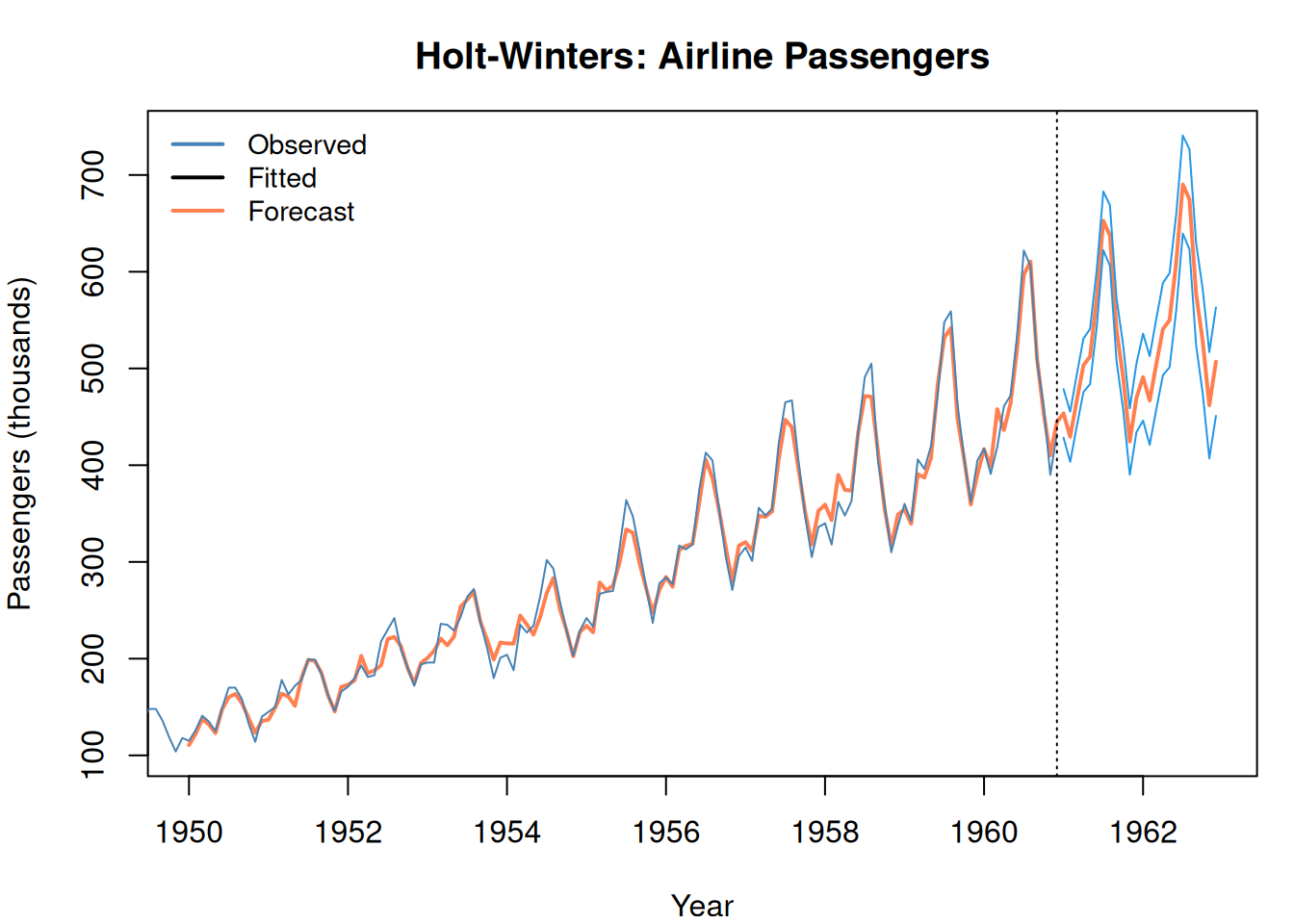
Figure 5: Holt-Winters captures trend AND seasonality

Which Exponential Smoothing to Use?

Does the data have a trend?
  |
  +-- No ──── Does it have seasonality?
  |             |
  |             +-- No ──── Simple ES (one parameter: α)
  |             +-- Yes ─── Seasonal ES
  |
  +-- Yes ─── Does it have seasonality?
                |
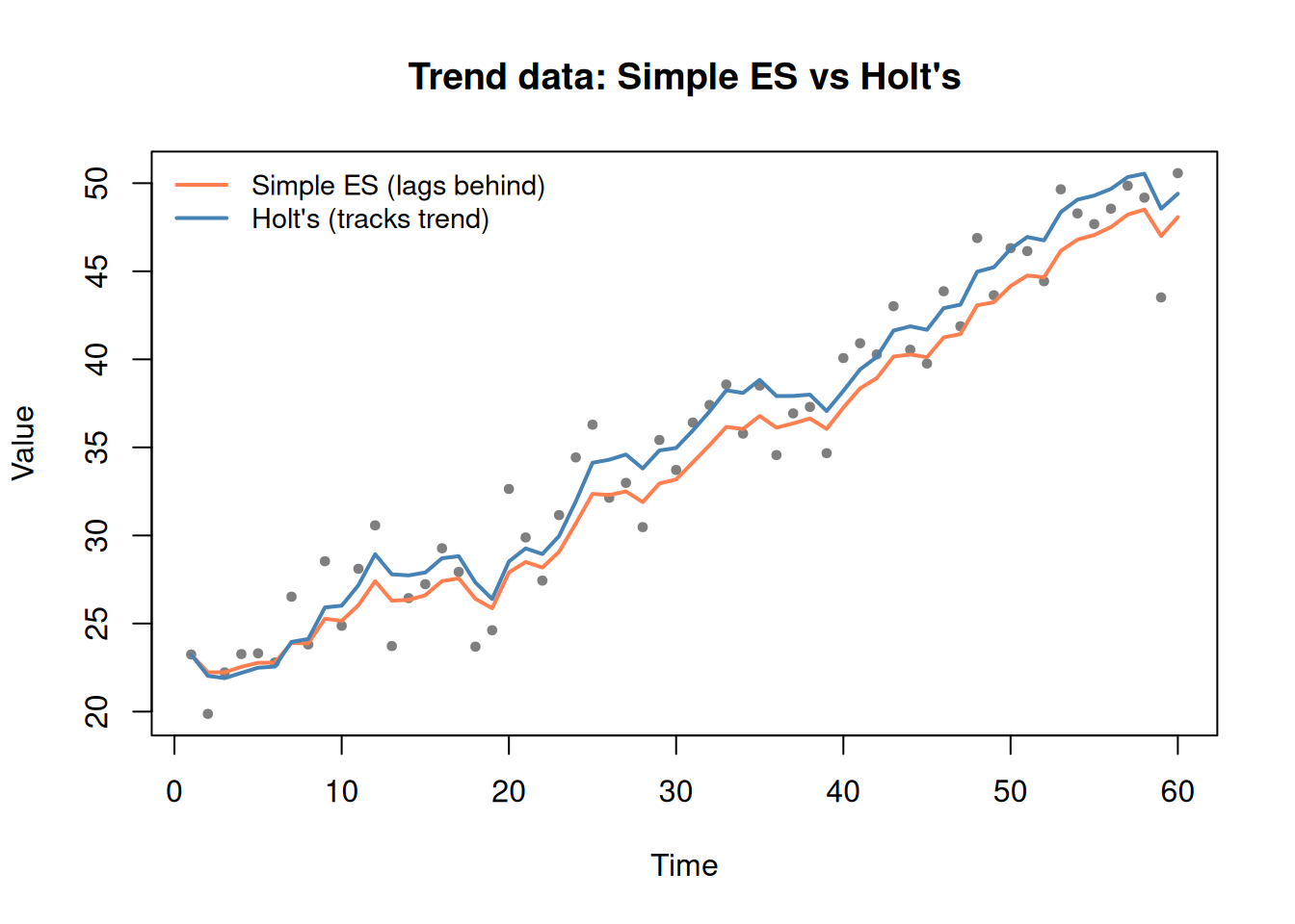
                +-- No ──── Holt (two parameters: α, β)
                +-- Yes ─── Holt-Winters (three parameters: α, β, γ)

5. All Parameters at a Glance

par(mfrow = c(1, 3), mar = c(4, 4, 3, 1))

set.seed(42)
n2 <- 50

# Alpha demo: level data with a jump
x_level <- c(rnorm(25, 50, 2), rnorm(25, 55, 2))
plot(1:n2, x_level, pch = 19, cex = 0.5, col = "gray50",
  main = "α controls level responsiveness",
  xlab = "Time", ylab = "Value")
lines(1:n2, ses(x_level, 0.1), col = "steelblue", lwd = 2)
lines(1:n2, ses(x_level, 0.9), col = "coral", lwd = 2)
legend("topleft", bty = "n", cex = 0.8,
  legend = c("α=0.1 (smooth)", "α=0.9 (reactive)"),
  col = c("steelblue", "coral"), lwd = 2)

# Beta demo: trending data
x_tr <- 10 + 0.8 * (1:n2) + rnorm(n2, 0, 2)
# Low beta
S1 <- Tr1 <- S2 <- Tr2 <- numeric(n2)
S1[1] <- S2[1] <- x_tr[1]; Tr1[1] <- Tr2[1] <- 0
for (t in 2:n2) {
  S1[t] <- 0.3 * x_tr[t] + 0.7 * (S1[t-1] + Tr1[t-1])
  Tr1[t] <- 0.1 * (S1[t] - S1[t-1]) + 0.9 * Tr1[t-1]
  S2[t] <- 0.3 * x_tr[t] + 0.7 * (S2[t-1] + Tr2[t-1])
  Tr2[t] <- 0.8 * (S2[t] - S2[t-1]) + 0.2 * Tr2[t-1]
}
plot(1:n2, x_tr, pch = 19, cex = 0.5, col = "gray50",
  main = "β controls trend responsiveness",
  xlab = "Time", ylab = "Value")
lines(1:n2, S1 + Tr1, col = "steelblue", lwd = 2)
lines(1:n2, S2 + Tr2, col = "coral", lwd = 2)
legend("topleft", bty = "n", cex = 0.8,
  legend = c("β=0.1 (stable trend)", "β=0.8 (reactive trend)"),
  col = c("steelblue", "coral"), lwd = 2)

# Gamma demo: seasonal data
x_seas <- 50 + rep(c(0, 5, 10, 5, 0, -5, -10, -5), 6) + rnorm(48, 0, 1.5)
ts_seas <- ts(x_seas, frequency = 8)
fit_lo <- HoltWinters(ts_seas, gamma = 0.1)

Warning in HoltWinters(ts_seas, gamma = 0.1): optimization difficulties: ERROR:
ABNORMAL_TERMINATION_IN_LNSRCH

fit_hi <- HoltWinters(ts_seas, gamma = 0.9)
plot(1:48, x_seas, pch = 19, cex = 0.5, col = "gray50",
  main = "γ controls seasonal responsiveness",
  xlab = "Time", ylab = "Value")
lines(9:48, fit_lo$fitted[, "xhat"], col = "steelblue", lwd = 2)
lines(9:48, fit_hi$fitted[, "xhat"], col = "coral", lwd = 2)
legend("topleft", bty = "n", cex = 0.8,
  legend = c("γ=0.1 (stable season)", "γ=0.9 (reactive season)"),
  col = c("steelblue", "coral"), lwd = 2)

par(mfrow = c(1, 1))

Figure 6: What each smoothing parameter controls

How to choose α, β, γ? Cross-validation (Module 3) — try different values, pick the ones that minimize forecast error on held-out data. R’s HoltWinters() does this automatically.

6. ARIMA: A Different Approach

Exponential smoothing is intuitive but limited in the patterns it can express. ARIMA is more flexible — it combines three ideas into one framework.

ARIMA(p, d, q) — What the Letters Mean

Letter	Name	What it does
p	AutoRegressive order	Use the last \(p\) values to predict the next
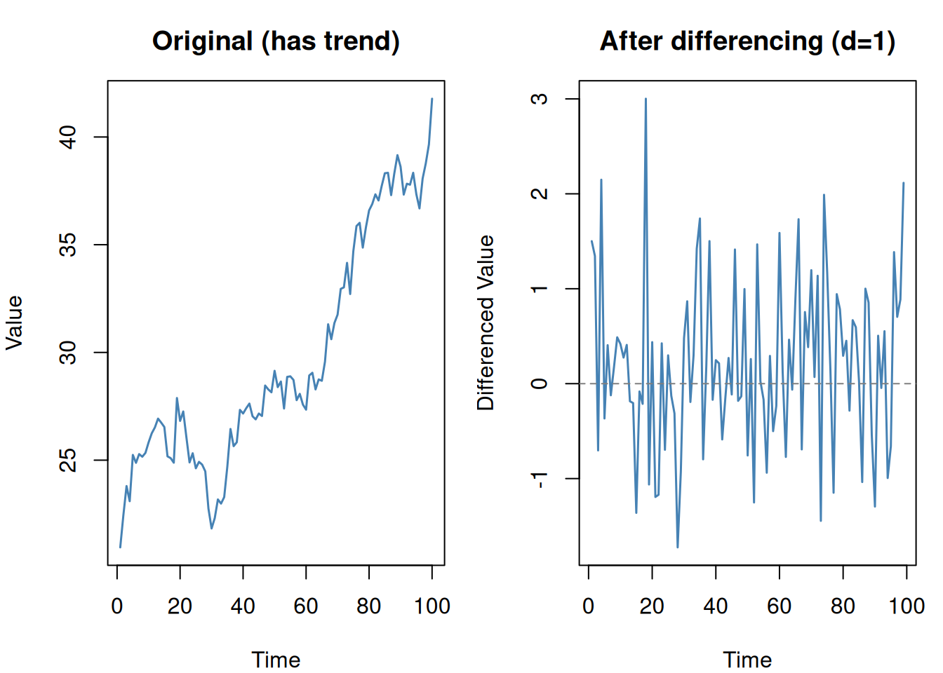
d	Differencing order	How many times to difference the data to remove trend
q	Moving Average order	Use the last \(q\) forecast errors to correct predictions

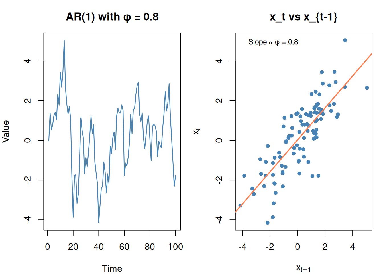
AR: Autoregressive (the “p” part)

Tomorrow’s value depends on today’s value (and maybe yesterday’s):

\[x_t = c + \phi_1 x_{t-1} + \phi_2 x_{t-2} + \dots + \phi_p x_{t-p} + \epsilon_t\]

Like regression, but instead of predicting from other variables, you predict from your own past values.

set.seed(42)
n3 <- 100

# AR(1) process
ar_data <- numeric(n3)
ar_data[1] <- 0
phi <- 0.8

for (t in 2:n3) {
  ar_data[t] <- phi * ar_data[t - 1] + rnorm(1, 0, 1)
}

par(mfrow = c(1, 2), mar = c(4, 4, 3, 1))

plot(1:n3, ar_data, type = "l", col = "steelblue", lwd = 1.5,
  main = paste0("AR(1) with φ = ", phi),
  xlab = "Time", ylab = "Value")

# Show the relationship: x_t vs x_{t-1}
plot(ar_data[1:(n3-1)], ar_data[2:n3],
  pch = 19, cex = 0.8, col = "steelblue",
  main = "x_t vs x_{t-1}",
  xlab = expression(x[t-1]), ylab = expression(x[t]))
abline(lm(ar_data[2:n3] ~ ar_data[1:(n3-1)]), col = "coral", lwd = 2)
legend("topleft", bty = "n", cex = 0.8,
  legend = paste0("Slope ≈ φ = ", round(cor(ar_data[1:(n3-1)], ar_data[2:n3]), 2)))

par(mfrow = c(1, 1))

Figure 7: AR(1): each value depends on the previous one, plus noise

I: Integrated / Differencing (the “d” part)

ARIMA requires stationary data (no trend, constant variance). If your data has a trend, differencing removes it:

\[x_t' = x_t - x_{t-1}\]

# Trending data
x_trended <- 20 + 0.3 * (1:n3) + cumsum(rnorm(n3, 0, 1))
x_diffed <- diff(x_trended)

par(mfrow = c(1, 2), mar = c(4, 4, 3, 1))

plot(1:n3, x_trended, type = "l", col = "steelblue", lwd = 1.5,
  main = "Original (has trend)",
  xlab = "Time", ylab = "Value")

plot(1:(n3-1), x_diffed, type = "l", col = "steelblue", lwd = 1.5,
  main = "After differencing (d=1)",
  xlab = "Time", ylab = "Differenced Value")
abline(h = 0, lty = 2, col = "gray50")

par(mfrow = c(1, 1))

Figure 8: Differencing removes trend, making the data stationary

• d = 0: Data is already stationary (no trend)
• d = 1: Difference once (removes linear trend)
• d = 2: Difference twice (removes quadratic trend) — rarely needed

MA: Moving Average (the “q” part)

Tomorrow’s value depends on today’s forecast error:

\[x_t = c + \epsilon_t + \theta_1 \epsilon_{t-1} + \theta_2 \epsilon_{t-2} + \dots + \theta_q \epsilon_{t-q}\]

This corrects systematic patterns in the errors. If you keep over-predicting, the MA term adjusts.

Putting It Together

ARIMA(1,1,1) means: difference once, then model with 1 AR term and 1 MA term.

# Fit ARIMA to airline passengers
fit_arima <- arima(AirPassengers, order = c(1, 1, 1),
                   seasonal = list(order = c(1, 1, 1), period = 12))

# Forecast
pred_arima <- predict(fit_arima, n.ahead = 24)

par(mar = c(4, 4, 3, 1))
ts.plot(AirPassengers, pred_arima$pred,
  col = c("steelblue", "coral"), lwd = c(1.5, 2),
  main = "ARIMA Forecast: Airline Passengers",
  ylab = "Passengers (thousands)")

# Confidence interval
upper <- pred_arima$pred + 1.96 * pred_arima$se
lower <- pred_arima$pred - 1.96 * pred_arima$se
time_pred <- time(pred_arima$pred)
polygon(c(time_pred, rev(time_pred)), c(upper, rev(lower)),
  col = adjustcolor("coral", 0.2), border = NA)

legend("topleft", bty = "n",
  legend = c("Observed", "Forecast", "95% CI"),
  col = c("steelblue", "coral", adjustcolor("coral", 0.3)),
  lwd = c(2, 2, 8), cex = 0.9)

Figure 9: ARIMA automatically selects p, d, q and forecasts ahead

7. ARIMA vs Exponential Smoothing: When to Use Which

	Exponential Smoothing	ARIMA
Simplicity	Simpler, fewer parameters	More complex, flexible
Data needed	Works with shorter series	Needs ~40+ observations
Noisy/volatile data	More robust	Can struggle with outliers
Complex patterns	Limited to level/trend/season	Can model many patterns
Interpretability	Parameters have clear meaning	p, d, q less intuitive
Special case	Simple ES	= ARIMA(0,1,1)

TipPractical Rule of Thumb

• Short, noisy, volatile data → exponential smoothing
• Long, stable data with many observations → ARIMA
• When in doubt → try both, pick the one with lower cross-validated error

8. GARCH: Forecasting How MUCH Things Will Vary

Everything above forecasts the value — what will the temperature be tomorrow? GARCH answers a different question: how volatile will it be?

Think of stock markets: some weeks are calm, some are wild. The actual price might be unpredictable, but the amount of volatility has patterns.

\[\sigma_t^2 = \omega + \alpha_1 \epsilon_{t-1}^2 + \beta_1 \sigma_{t-1}^2\]

Symbol	What it is	Plain English
\(\sigma_t^2\)	Predicted variance at time \(t\)	How much volatility we expect
\(\omega\)	Baseline variance	The minimum level of volatility
\(\epsilon_{t-1}^2\)	Previous squared error	How big yesterday’s surprise was
\(\alpha_1\)	Shock sensitivity	How much a single surprise increases future volatility
\(\beta_1\)	Persistence	How long volatility stays elevated after a shock
\(\sigma_{t-1}^2\)	Previous variance	Yesterday’s volatility forecast

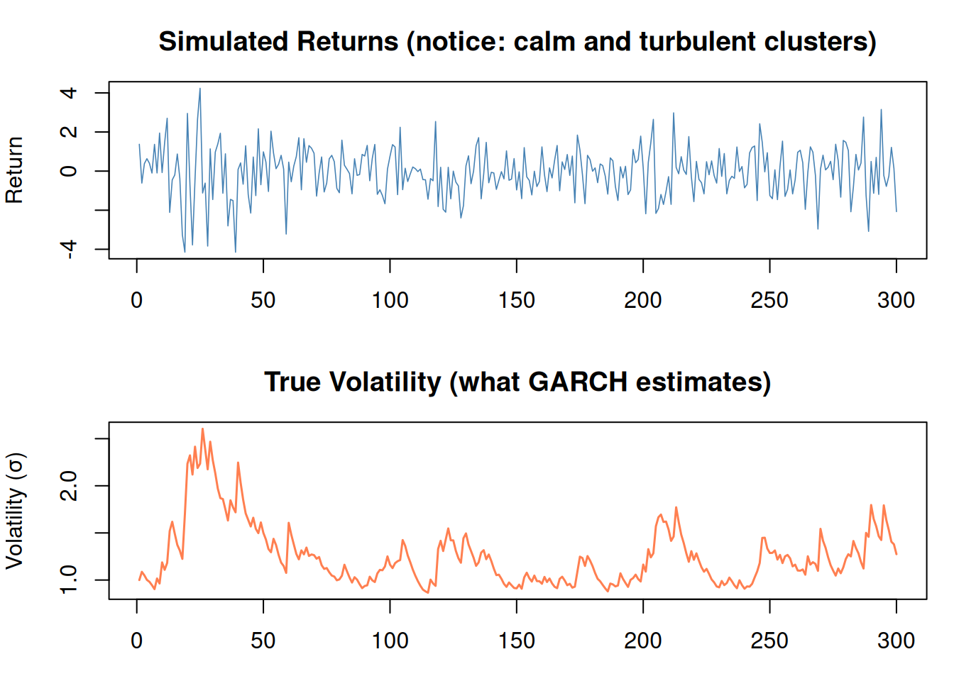
Key insight: \(\alpha\) captures shocks (a big surprise today → more volatility tomorrow). \(\beta\) captures persistence (volatility tends to stay high once it’s high).

set.seed(42)

# Simulate GARCH-like data
n4 <- 300
returns <- numeric(n4)
vol <- numeric(n4)
omega <- 0.1
alpha_g <- 0.15
beta_g <- 0.8

vol[1] <- 1
returns[1] <- rnorm(1, 0, sqrt(vol[1]))

for (t in 2:n4) {
  vol[t] <- omega + alpha_g * returns[t-1]^2 + beta_g * vol[t-1]
  returns[t] <- rnorm(1, 0, sqrt(vol[t]))
}

par(mfrow = c(2, 1), mar = c(3, 4, 3, 1))

plot(1:n4, returns, type = "l", col = "steelblue", lwd = 0.8,
  main = "Simulated Returns (notice: calm and turbulent clusters)",
  ylab = "Return", xlab = "")

plot(1:n4, sqrt(vol), type = "l", col = "coral", lwd = 1.5,
  main = "True Volatility (what GARCH estimates)",
  ylab = "Volatility (σ)", xlab = "Time")

par(mfrow = c(1, 1))

Figure 10: Volatility clusters: calm periods and turbulent periods alternate

When to Use GARCH

A common practice check asks whether you know the difference:

Question asks about…	Use
“Forecast the value”	Exponential smoothing or ARIMA
“Forecast volatility/risk/variance”	GARCH
“Predict how much values will fluctuate”	GARCH
“Build confidence intervals that change over time”	GARCH
“Portfolio risk” or “Value at Risk”	GARCH

9. The Complete Decision Tree

What are you forecasting?
  |
  +-- The VALUE itself ──── Is there a trend? Seasonality?
  |                           |
  |                           +-- Level only ────────── Simple ES
  |                           +-- Level + trend ─────── Double ES (Holt)
  |                           +-- Level + trend + season ── Triple ES (Holt-Winters)
  |                           +-- Complex pattern, lots of data ── ARIMA
  |
  +-- The VOLATILITY/VARIANCE ── GARCH
  |
  +-- Has something CHANGED? ── CUSUM (Module 6)

10. Cheat Sheet: The Whole Story on One Page

TIME SERIES FORECASTING RECIPE
================================

EXPONENTIAL SMOOTHING
---------------------
Simple:   Sₜ = α·xₜ + (1-α)·Sₜ₋₁                    [level only]
Holt:     + Tₜ = β·(Sₜ - Sₜ₋₁) + (1-β)·Tₜ₋₁         [+ trend]
H-W:      + Cₜ = γ·(xₜ/Sₜ) + (1-γ)·Cₜ₋ₗ              [+ seasonality]

Parameters:
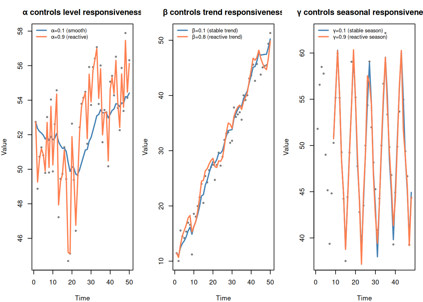
  α → level responsiveness    (high = reactive, low = smooth)
  β → trend responsiveness
  γ → seasonal responsiveness
  All chosen via cross-validation

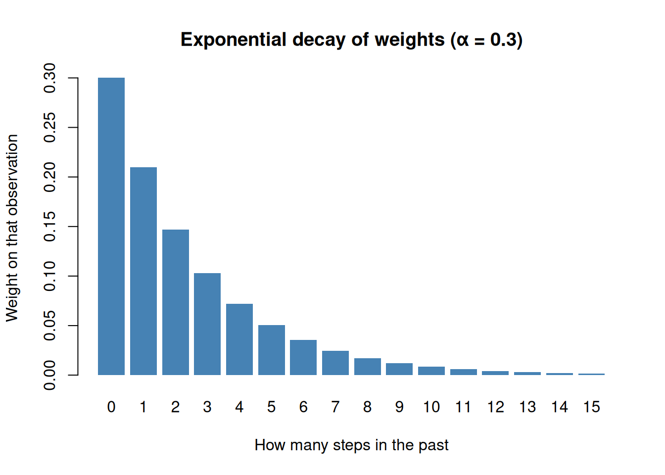
"Exponential" = past data gets exponentially decaying weights

ARIMA(p, d, q)
--------------
p = autoregressive terms  (predict from past values)
d = differencing           (remove trend)
q = moving average terms   (correct from past errors)

ARIMA(0,1,1) = simple exponential smoothing
Use when: stable data, 40+ observations, complex patterns

GARCH(p, q)
-----------
σₜ² = ω + α·εₜ₋₁² + β·σₜ₋₁²

Forecasts VARIANCE, not value.
Use when: "volatility", "risk", "how much will values vary"

PRACTICAL DECISION:
  "Forecast the value" → ES or ARIMA
  "Forecast the variance/volatility" → GARCH
  "Detect a change" → CUSUM

11. Check Your Understanding

NoteTest Yourself

Before moving on, try to answer these without scrolling up:

1. What does \(\alpha\) control in exponential smoothing? What happens when you increase it?
2. Why is it called “exponential” smoothing?
3. When do you need Holt’s method instead of simple ES?
4. What does the “d” in ARIMA stand for, and why is it needed?
5. What is the key difference between ARIMA and exponential smoothing? When would you prefer each?
6. GARCH forecasts _______, not _______. (Fill in the blanks.)
7. A manager asks you to “predict next quarter’s sales.” Which method? Now they ask “predict how volatile next quarter’s sales will be.” Which method?
8. What is ARIMA(0,1,1) equivalent to?
9. Data has 20 observations, lots of noise, and a seasonal pattern. Exponential smoothing or ARIMA? Why?