Simulation & Markov: Probability Models for Real Systems

Distributions, QQ plots, M/M/1 queues, and steady states

The Big Picture

Most of this guide has been “throw data at a model.” This module inverts that: when the only thing you know about a data point is its value, a well-matched probability distribution can solve the problem without any feature engineering.

A useful opening story is a startup that wanted to resell empty season-ticket seats as upgrades. A big feature list (ticket holder demographics, weather, team record, opponent, day of week) looked inevitable — until the team realized fans tend to arrive at about the same relative position in the crowd every game. The deviation is approximately normal. A single distribution replaced the whole feature pipeline.

This demo walks through the distributions, QQ plots, a simple queuing simulation, and Markov-chain steady state — the four tools the module uses to reason about systems.

Tip

Rule of thumb: before engineering features, fit a distribution. If it fits, you may be done.

---

The Distributions You Should Recognize

Bernoulli → Binomial → Geometric

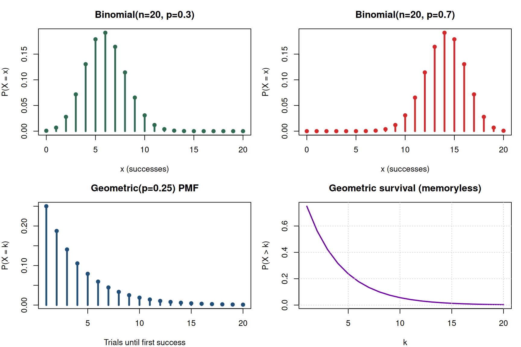
The Bernoulli trial is a single weighted coin flip. Chain \(n\) of them together and count successes → binomial. Ask how many until the first success → geometric.

Figure 1: Binomial PMFs for different p (top); Geometric PMF and survival function (bottom).

The binomial converges to the normal distribution as \(n\) grows, which is why the normal is so useful — it’s the large-\(n\) limit of so many counting processes.

The geometric is your “how many trials until X” tool. It doubles as a diagnostic: if you want to know whether at-bats are really i.i.d. Bernoulli trials, check whether at-bats-until-broken-bat fits a geometric distribution. If it does, you don’t need to model weather, pitcher, pitch type, batter — the independence assumption is already good enough.

Warning

Watch out: in the geometric distribution, \(p\) is the probability of the thing you’re waiting for. Sometimes that’s a good outcome (job offer), sometimes bad (defective unit). Define it explicitly every time — you’ll see this trap on practice checks.

Poisson ↔︎ Exponential (the same distribution in disguise)

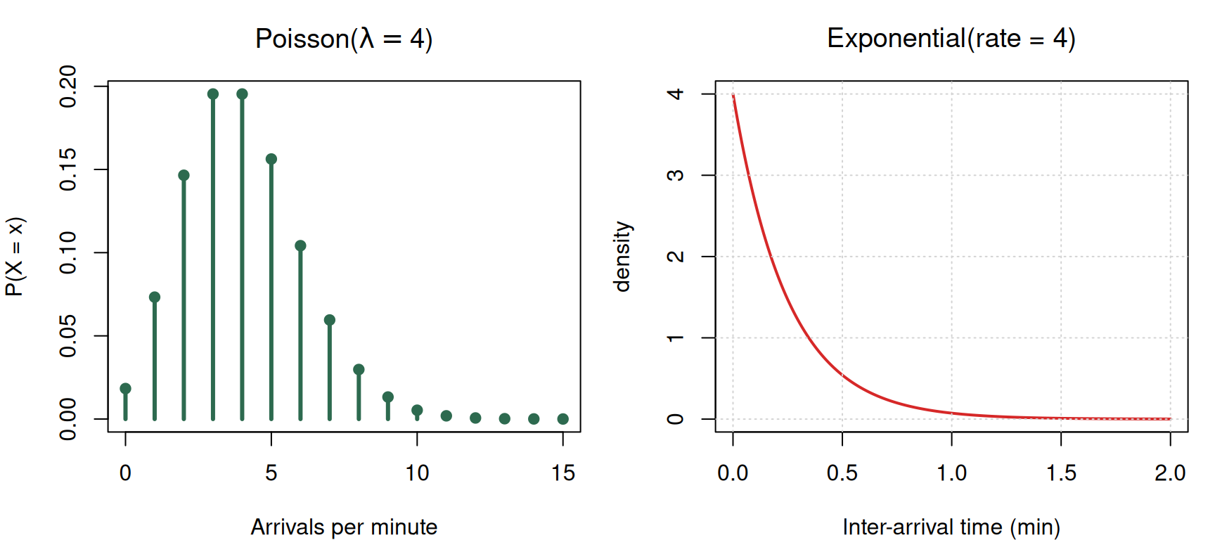
If customers arrive at an average rate \(\lambda\) per minute and arrivals are independent, the count in a fixed window is Poisson and the inter-arrival time is exponential with mean \(1/\lambda\). One distribution in time units, the other in count units.

Figure 2: Poisson PMF and the matching exponential density.

Weibull — failure rate that varies with age

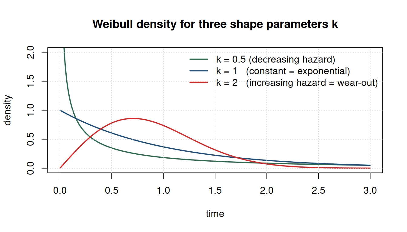
The Weibull is like the geometric, but continuous in time. Its shape parameter \(k\) controls whether the failure rate shrinks, stays flat, or grows.

Figure 3: Weibull density for k < 1 (weak parts fail first), k = 1 (exponential), k > 1 (wear-out).

Note

Check your understanding: Tires are more likely to fail the more miles they’ve been driven. Is this memoryless? Which distribution fits?

Answer: not memoryless (depends on history), so not exponential. Weibull with \(k > 1\) is the right tool.

---

QQ Plots — Sanity Check for Distribution Fit

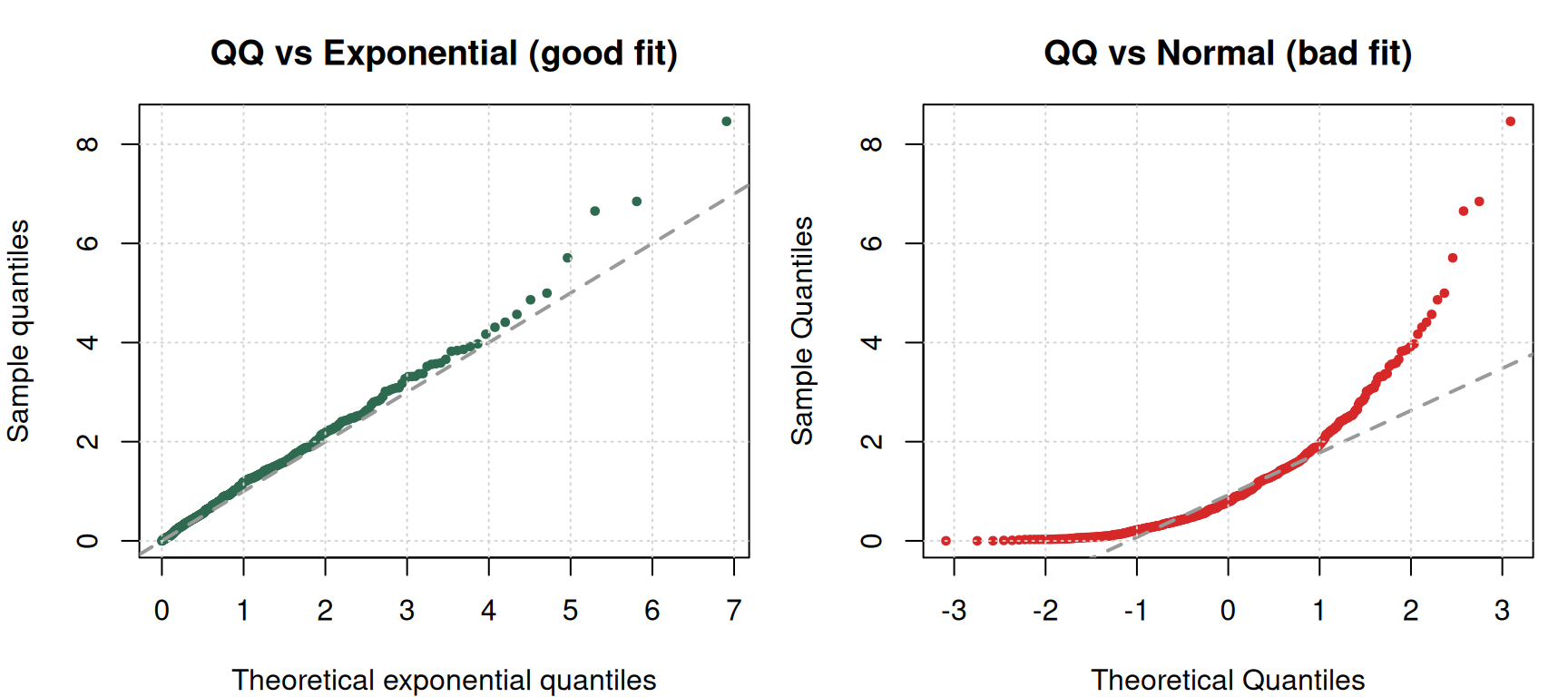
A statistical test collapses the fit to a single number. A QQ plot shows you where a distribution diverges from the data — which matters enormously if the tails are the point of your project.

Figure 4: QQ plots: (left) simulated exponential data vs theoretical exponential — nearly straight. (right) the same data vs theoretical normal — clearly bad, especially in the tails.

Tip

If the data and the theoretical distribution match, points fall on the 45° line. Where they drift off tells you the story — upper-tail heavier than normal, lower-tail compressed, etc.

---

Why Averages Aren’t Enough — A Queuing Simulation

A classic queueing example: wafers arrive at a semiconductor machine every 20 seconds on average; processing takes 19 seconds on average. Under these averages alone, the queue is always empty and throughput is effortless. Add Poisson arrivals and exponential service — same means — and the average queue explodes to ~19 wafers.

Let’s simulate it.

set.seed(1)

simulate_mm1 <- function(n_customers = 5000, lambda = 1 / 20, mu = 1 / 19) {
  inter_arrivals <- rexp(n_customers, rate = lambda)
  service_times  <- rexp(n_customers, rate = mu)

  arrival_time <- cumsum(inter_arrivals)
  start_time   <- numeric(n_customers)
  finish_time  <- numeric(n_customers)

  start_time[1]  <- arrival_time[1]
  finish_time[1] <- start_time[1] + service_times[1]

  for (i in 2:n_customers) {
    start_time[i]  <- max(arrival_time[i], finish_time[i - 1])
    finish_time[i] <- start_time[i] + service_times[i]
  }

  wait_time <- start_time - arrival_time
  data.frame(arrival_time, start_time, finish_time, wait_time)
}

sim <- simulate_mm1()
cat("Mean wait time (sec):", round(mean(sim$wait_time), 2), "\n")

Mean wait time (sec): 280.47 

cat("Max wait time  (sec):", round(max(sim$wait_time), 2), "\n")

Max wait time  (sec): 1212.84 

cat("Utilization (expected):", round((1 / 19) / (1 / 20), 3), "\n")

Utilization (expected): 1.053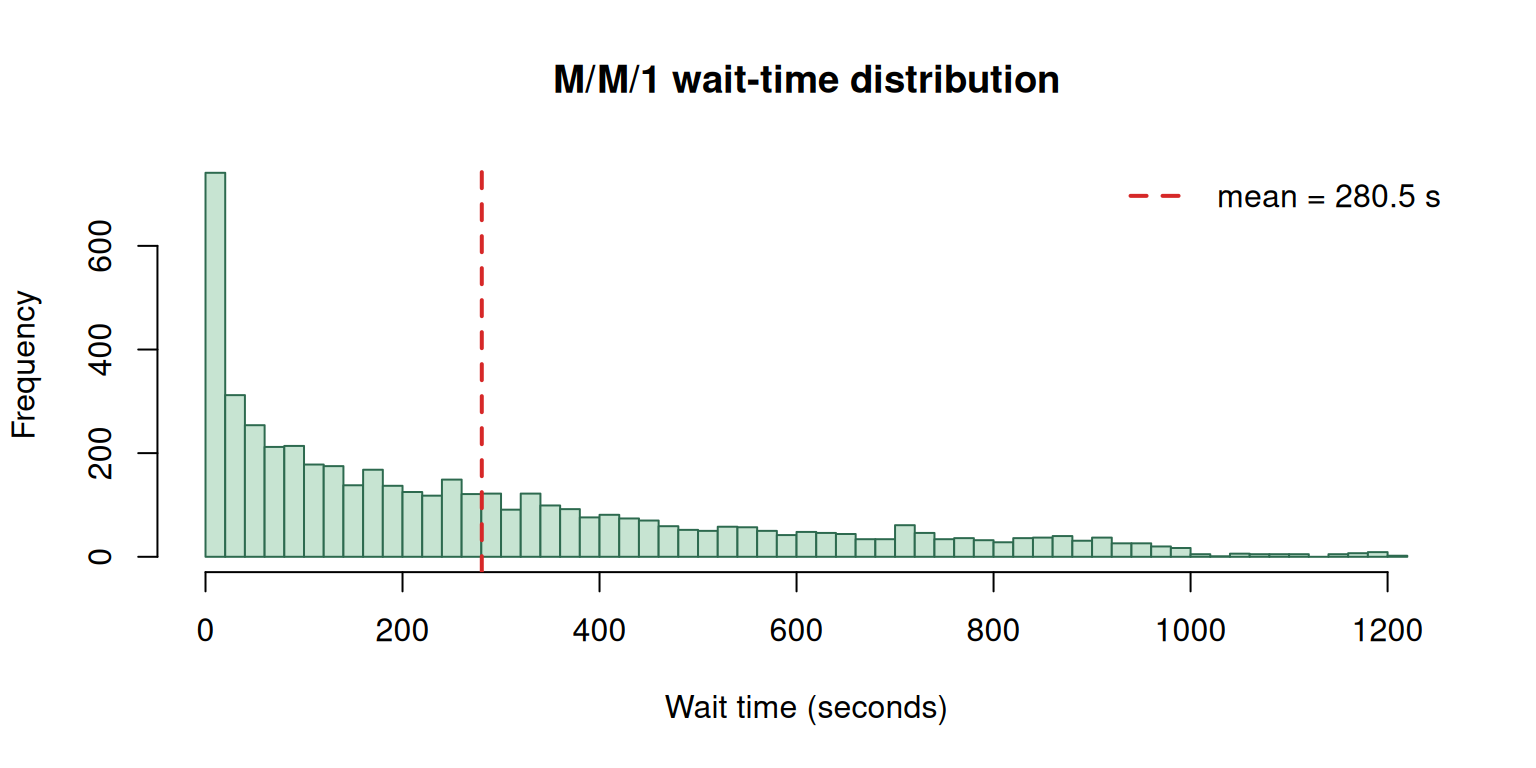 

Figure 5: Wait-time distribution for an M/M/1 queue with mean inter-arrival 20s and mean service 19s. Most waits are short but the tail is long — the average already disagrees with the ‘no queue’ story that averaging inputs would tell.

Warning

Common pitfall: “If arrivals average every 20 seconds and service takes 19 seconds, the queue is small.” This is wrong. Variability in inter-arrival and service times — even with those means — creates a substantial queue. Simulation exists precisely because averages can’t predict queue behavior once randomness enters.

---

Memorylessness — The Single Property That Makes the Math Tractable

The exponential distribution has one peculiar property: given that you’ve already waited \(s\) units, the distribution of remaining time is still exponential with the same rate. Past history is irrelevant.

set.seed(7)
samples <- rexp(50000, rate = 1)

# Unconditional
p_exceed_2 <- mean(samples > 2)

# Conditional: already waited 3, ask for 2 more
survived_3 <- samples[samples > 3]
p_exceed_3_plus_2 <- mean(survived_3 > 5)

cat("P(X > 2) unconditional:       ", round(p_exceed_2, 4), "\n")

P(X > 2) unconditional:        0.136 

cat("P(X > 5 | X > 3) conditional: ", round(p_exceed_3_plus_2, 4), "\n")

P(X > 5 | X > 3) conditional:  0.1268 

The two numbers are (approximately) the same. That’s what memorylessness means — and it’s why M/M/1 queues admit closed-form solutions. Tire failure, by contrast, is history-dependent (worn tires fail faster), so tires cannot be modeled as exponential — Weibull with \(k > 1\) is the right tool.

---

Markov Chains — Steady State via Eigen-Decomposition

A Markov chain has a finite set of states and a transition matrix \(P\) where \(P_{ij}\) is the probability of moving from state \(i\) to state \(j\) in one step. Starting with an initial distribution \(\pi\), the distribution after \(k\) steps is \(\pi P^k\). The steady-state distribution \(\pi^*\) is the one that doesn’t change: \(\pi^* P = \pi^*\) with \(\sum \pi_i^* = 1\).

Mathematically, \(\pi^*\) is the left eigenvector of \(P\) with eigenvalue 1.

# Classic weather example: Sunny / Cloudy / Rainy
states <- c("Sunny", "Cloudy", "Rainy")
P <- matrix(c(
  0.70, 0.20, 0.10,   # from Sunny
  0.30, 0.40, 0.30,   # from Cloudy
  0.20, 0.45, 0.35    # from Rainy
), nrow = 3, byrow = TRUE)
rownames(P) <- colnames(P) <- states
P

       Sunny Cloudy Rainy
Sunny    0.7   0.20  0.10
Cloudy   0.3   0.40  0.30
Rainy    0.2   0.45  0.35

# Eigen decomposition of P^T — the left eigenvector of P is the right eigenvector of P^T
eig <- eigen(t(P))

# Find the eigenvector corresponding to eigenvalue ~ 1
idx <- which.min(abs(eig$values - 1))
pi_star_raw <- Re(eig$vectors[, idx])
pi_star <- pi_star_raw / sum(pi_star_raw)
names(pi_star) <- states
round(pi_star, 4)

 Sunny Cloudy  Rainy 
0.4636 0.3182 0.2182 

# Verify by simulation: start in Sunny, take many steps, record visit fractions
set.seed(42)
n_steps <- 100000
state <- 1L  # start in Sunny
visits <- integer(3)

for (step in seq_len(n_steps)) {
  visits[state] <- visits[state] + 1L
  state <- sample.int(3, size = 1, prob = P[state, ])
}

empirical <- visits / n_steps
names(empirical) <- states
round(empirical, 4)

 Sunny Cloudy  Rainy 
0.4629 0.3183 0.2188 

The eigen-decomposition and the empirical random walk agree — that’s the Markov-chain steady state.

Note

Check your understanding: Real weather is not actually a good Markov example — real weather is highly history-dependent. Why bother with Markov chains at all?

Answer: applications like PageRank (ranking web pages by random-walk steady state), LRMC college basketball rankings, urban sprawl, and long-run disease modeling. In these cases the system isn’t literally memoryless short-term, but over long horizons the memorylessness assumption washes out and the steady state still gives useful rankings.

---

PageRank — One Matrix Multiply

PageRank treats the web as a graph: each page is a state, and the transition probability from page \(i\) to page \(j\) is proportional to whether \(i\) links to \(j\). The steady-state distribution tells you how often a random walker lands on each page — Google’s original ranking signal.

# Tiny web of 5 pages
link_matrix <- matrix(0, nrow = 5, ncol = 5)
# Page 1 links to 2, 3
link_matrix[1, c(2, 3)] <- 1
# Page 2 links to 3
link_matrix[2, 3] <- 1
# Page 3 links to 1, 4
link_matrix[3, c(1, 4)] <- 1
# Page 4 links to 3, 5
link_matrix[4, c(3, 5)] <- 1
# Page 5 links to 3
link_matrix[5, 3] <- 1

# Row-normalize to get transition matrix
P_web <- link_matrix / rowSums(link_matrix)

# Steady-state via eigen
eig_web <- eigen(t(P_web))
rank_raw <- Re(eig_web$vectors[, which.min(abs(eig_web$values - 1))])
page_rank <- rank_raw / sum(rank_raw)
names(page_rank) <- paste0("Page", 1:5)
sort(round(page_rank, 4), decreasing = TRUE)

Page3 Page1 Page4 Page2 Page5 
  0.4   0.2   0.2   0.1   0.1 

Page 3 dominates — it receives links from almost every other page, so a random walker gets funneled there.

---

Cheat Sheet

Situation	Distribution / tool
Single yes/no trial	Bernoulli
Count of successes in \(n\) trials	Binomial
Trials until first success	Geometric
Arrivals in a fixed window	Poisson
Time between arrivals (memoryless)	Exponential
Time to failure (age-dependent)	Weibull (\(k \ne 1\))
Visual distribution fit	QQ plot
Queue with closed-form math	M/M/1 (needs exponential)
Queue with arbitrary complexity	Simulation
Long-run rankings over a transition graph	Markov chain steady state

Warning

Common pitfalls recap:

1. Averages ≠ queues. Variability makes lines even when \(\lambda < \mu\).
2. Geometric \(p\) direction. Define \(p\) as the thing you’re waiting for, not always “success.”
3. Exponential only when memoryless. If history matters, use Weibull.
4. Weibull k = 1 reduces to exponential. Software reporting “best fit Weibull \(k = 1.002\)” is probably just fitting noise.
5. Markov chains need irreducibility. A steady state may not exist if states can’t reach each other.