Cross-Validation From Scratch: Why Testing on Training Data Is Cheating

The one technique every model depends on

1. The Problem: How Good Is Your Model, Really?

You build a model. It predicts your training data perfectly. Is it good?

No. It might have just memorized the data. A model that memorizes is useless on new data — like a student who memorizes answers but can’t solve new problems.

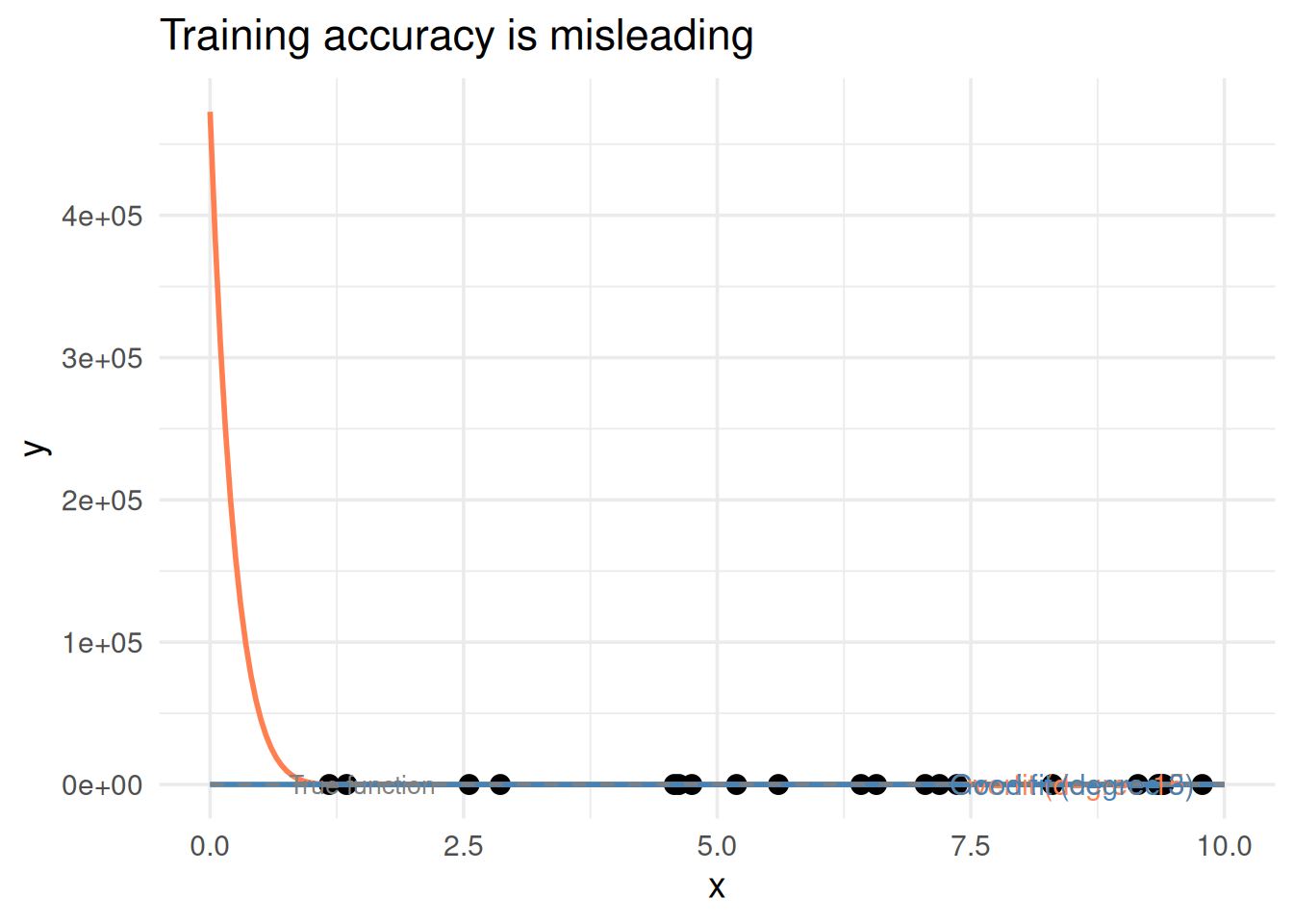
library(ggplot2)
set.seed(42)

# True relationship: simple curve
x <- sort(runif(20, 0, 10))
y <- 2 * sin(x) + rnorm(20, 0, 0.8)
df <- data.frame(x = x, y = y)

# Overfit model: high-degree polynomial
fit_over <- lm(y ~ poly(x, 15), data = df)
# Good model: low-degree polynomial
fit_good <- lm(y ~ poly(x, 3), data = df)

x_grid <- seq(0, 10, length.out = 200)
pred_over <- predict(fit_over, newdata = data.frame(x = x_grid))
pred_good <- predict(fit_good, newdata = data.frame(x = x_grid))

ggplot(df, aes(x, y)) +
  geom_point(size = 3) +
  geom_line(data = data.frame(x = x_grid, y = pred_over),
            aes(x, y), color = "coral", linewidth = 1) +
  geom_line(data = data.frame(x = x_grid, y = pred_good),
            aes(x, y), color = "steelblue", linewidth = 1) +
  geom_line(data = data.frame(x = x_grid, y = 2 * sin(x_grid)),
            aes(x, y), color = "gray50", linetype = "dashed") +
  annotate("text", x = 8.5, y = 4, label = "Overfit (degree 15)",
           color = "coral", size = 4) +
  annotate("text", x = 8.5, y = -1, label = "Good fit (degree 3)",
           color = "steelblue", size = 4) +
  annotate("text", x = 1.5, y = -2.5, label = "True function",
           color = "gray50", size = 3.5) +
  theme_minimal(base_size = 14) +
  labs(x = "x", y = "y", title = "Training accuracy is misleading")

Figure 1: The wiggly model fits training data perfectly but is clearly wrong

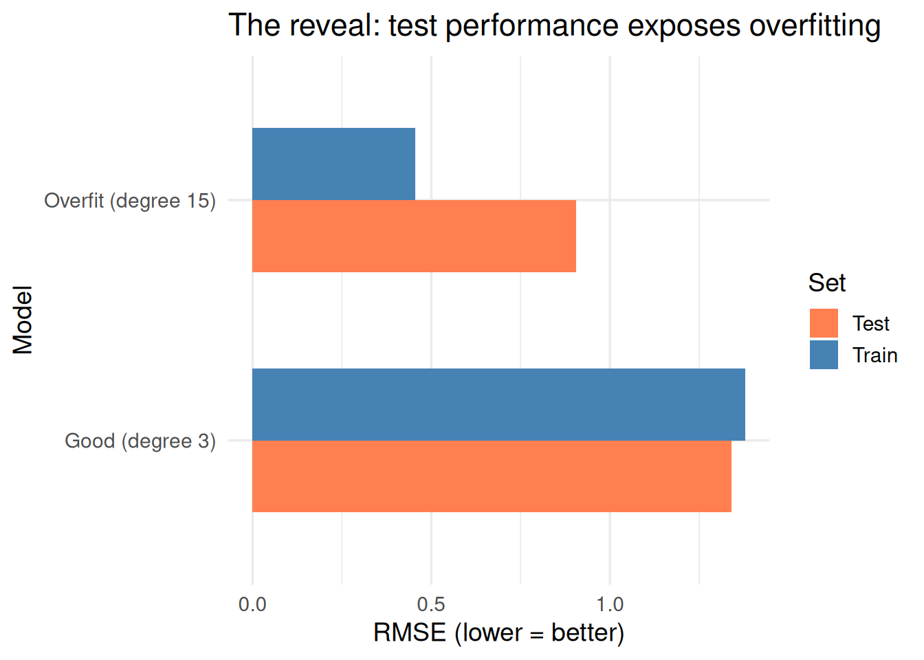
The red line hits every point — 100% training accuracy. But it’s wildly wrong between the points. The blue line misses some points but captures the real pattern.

How do we tell the difference? We need data the model has never seen.

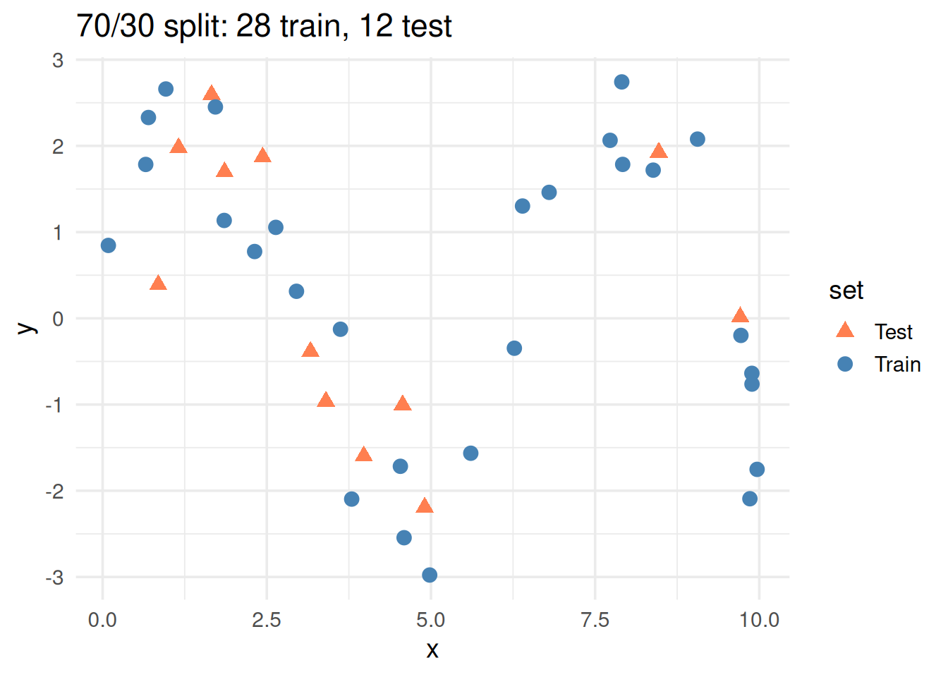
2. The Simplest Fix: Train/Test Split

Split your data into two pieces:

Training set (~70-80%): build the model
Test set (~20-30%): evaluate the model

The model never sees the test data during training. Its performance on the test set tells you how it will do on genuinely new data.

set.seed(7)
n <- 40
x_all <- sort(runif(n, 0, 10))
y_all <- 2 * sin(x_all) + rnorm(n, 0, 0.8)

# Random 70/30 split
train_idx <- sample(n, round(0.7 * n))
test_idx <- setdiff(1:n, train_idx)

df_all <- data.frame(
  x = x_all, y = y_all,
  set = ifelse(1:n %in% train_idx, "Train", "Test")
)

ggplot(df_all, aes(x, y, color = set, shape = set)) +
  geom_point(size = 3) +
  scale_color_manual(values = c("coral", "steelblue")) +
  scale_shape_manual(values = c(17, 19)) +
  theme_minimal(base_size = 14) +
  labs(x = "x", y = "y",
    title = paste0("70/30 split: ", length(train_idx), " train, ",
                   length(test_idx), " test"))

Figure 2: Split data into training (build the model) and test (evaluate it)

df_train <- df_all[df_all$set == "Train", ]
df_test <- df_all[df_all$set == "Test", ]

# Overfit
fit_over <- lm(y ~ poly(x, 15), data = df_train)
# Good
fit_good <- lm(y ~ poly(x, 3), data = df_train)

# Errors
results <- data.frame(
  Model = rep(c("Overfit (degree 15)", "Good (degree 3)"), each = 2),
  Set = rep(c("Train", "Test"), 2),
  RMSE = c(
    sqrt(mean(residuals(fit_over)^2)),
    sqrt(mean((df_test$y - predict(fit_over, df_test))^2)),
    sqrt(mean(residuals(fit_good)^2)),
    sqrt(mean((df_test$y - predict(fit_good, df_test))^2))
  )
)

ggplot(results, aes(x = Model, y = RMSE, fill = Set)) +
  geom_col(position = "dodge", width = 0.6) +
  scale_fill_manual(values = c("coral", "steelblue")) +
  theme_minimal(base_size = 14) +
  labs(y = "RMSE (lower = better)", title = "The reveal: test performance exposes overfitting") +
  coord_flip()

Figure 3: Overfit model: great on train, terrible on test. Good model: consistent on both.

The overfit model looks amazing on training data but falls apart on test data. The good model performs consistently on both.

The Problem with a Single Split

But there’s a catch: which 30% you hold out matters. A different random split gives a different score. Your evaluation depends on luck.

set.seed(1)
scores <- sapply(1:20, function(i) {
  idx <- sample(n, round(0.7 * n))
  train <- data.frame(x = x_all[idx], y = y_all[idx])
  test <- data.frame(x = x_all[-idx], y = y_all[-idx])
  fit <- lm(y ~ poly(x, 3), data = train)
  sqrt(mean((test$y - predict(fit, test))^2))
})

ggplot(data.frame(trial = 1:20, rmse = scores), aes(trial, rmse)) +
  geom_col(fill = "steelblue", alpha = 0.7) +
  geom_hline(yintercept = mean(scores), color = "coral", linewidth = 1, linetype = "dashed") +
  annotate("text", x = 17, y = mean(scores) + 0.1,
           label = paste0("Average: ", round(mean(scores), 2)),
           color = "coral", size = 4) +
  theme_minimal(base_size = 14) +
  labs(x = "Random Split #", y = "Test RMSE",
       title = "Same model, 20 different splits → 20 different scores")

Figure 4: Different random splits give different test scores — which one is ‘right’?

Solution: Don’t do one split. Do many splits and average. That’s cross-validation.

3. Cross-Validation: The Core Idea

k-Fold Cross-Validation

Divide data into \(k\) equal folds (groups)
Use fold 1 as test, train on folds 2-5 → get score 1
Use fold 2 as test, train on folds 1,3-5 → get score 2
… repeat for all folds
Average all \(k\) scores

Every point gets to be in the test set exactly once.

# Visual diagram of k-fold CV
k <- 5
fold_colors <- c("coral", "steelblue")

par(mar = c(2, 6, 3, 2))
plot(NULL, xlim = c(0, k), ylim = c(0.5, k + 0.5),
     xlab = "", ylab = "", xaxt = "n", yaxt = "n",
     main = "5-Fold Cross-Validation")

for (round in 1:k) {
  for (fold in 1:k) {
    col <- ifelse(fold == round,
      adjustcolor("coral", 0.8),
      adjustcolor("steelblue", 0.4))
    rect(fold - 1, k - round + 0.6, fold, k - round + 1.4, col = col, border = "white", lwd = 2)
    label <- ifelse(fold == round, "TEST", "train")
    text(fold - 0.5, k - round + 1, label, cex = 0.9,
         col = ifelse(fold == round, "white", "white"),
         font = ifelse(fold == round, 2, 1))
  }
  text(-0.3, k - round + 1, paste("Round", round), cex = 0.8, adj = 1)
}

text(k / 2, 0.3, "→ Average all 5 scores = cross-validation estimate", cex = 1, font = 2)

Figure 5: 5-fold cross-validation: each fold takes a turn as the test set

The Formula

The cross-validation estimate of model performance is just the average error across all folds:

\[\text{CV}(k) = \frac{1}{k} \sum_{i=1}^{k} \text{Error}_i\]

Symbol	What it is	Plain English
\(k\)	Number of folds	How many splits you make
\(\text{Error}_i\)	Error on fold \(i\) when it’s the test set	How badly the model did on that fold
\(\text{CV}(k)\)	Cross-validation score	The averaged, reliable performance estimate

For classification, “Error” is usually misclassification rate (% wrong). For regression, it’s usually RMSE or MSE.

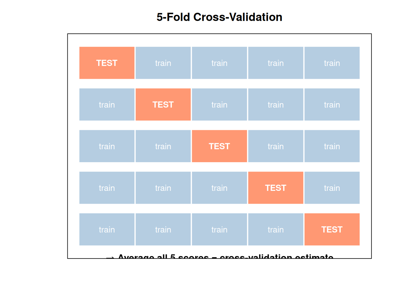
4. Choosing k (the Number of Folds)

Confusing but important: this \(k\) is different from KNN’s \(k\). This is the number of folds, not the number of neighbors.

Folds	Name	Train size	Test size	Pros	Cons
5	5-fold	80%	20%	Fast, good balance	Moderate variance
10	10-fold	90%	10%	Better estimate	Slower
\(n\)	Leave-one-out (LOO)	\(n-1\)	1	Uses max training data	Very slow, high variance

set.seed(42)
n <- 50
x <- sort(runif(n, 0, 10))
y <- 2 * sin(x) + rnorm(n, 0, 0.8)
df_cv <- data.frame(x = x, y = y)

# Run k-fold CV for different k values, repeat to see variance
fold_vals <- c(3, 5, 10, 25, n)
fold_labels <- c("3", "5", "10", "25", paste0(n, "\n(LOO)"))

results_list <- list()
for (fi in seq_along(fold_vals)) {
  kf <- fold_vals[fi]
  scores <- sapply(1:30, function(rep) {
    folds <- sample(rep(1:kf, length.out = n))
    errs <- sapply(1:kf, function(f) {
      train <- df_cv[folds != f, ]
      test <- df_cv[folds == f, ]
      if (nrow(train) < 4 || nrow(test) < 1) return(NA)
      fit <- lm(y ~ poly(x, 3), data = train)
      mean((test$y - predict(fit, test))^2)
    })
    mean(errs, na.rm = TRUE)
  })
  results_list[[fi]] <- data.frame(
    folds = fold_labels[fi],
    score = scores
  )
}

results_all <- do.call(rbind, results_list)
results_all$folds <- factor(results_all$folds, levels = fold_labels)

ggplot(results_all, aes(folds, score)) +
  geom_boxplot(fill = "steelblue", alpha = 0.6, outlier.size = 1) +
  theme_minimal(base_size = 14) +
  labs(x = "Number of Folds", y = "CV Score (MSE)",
       title = "More folds = less variance in the estimate")

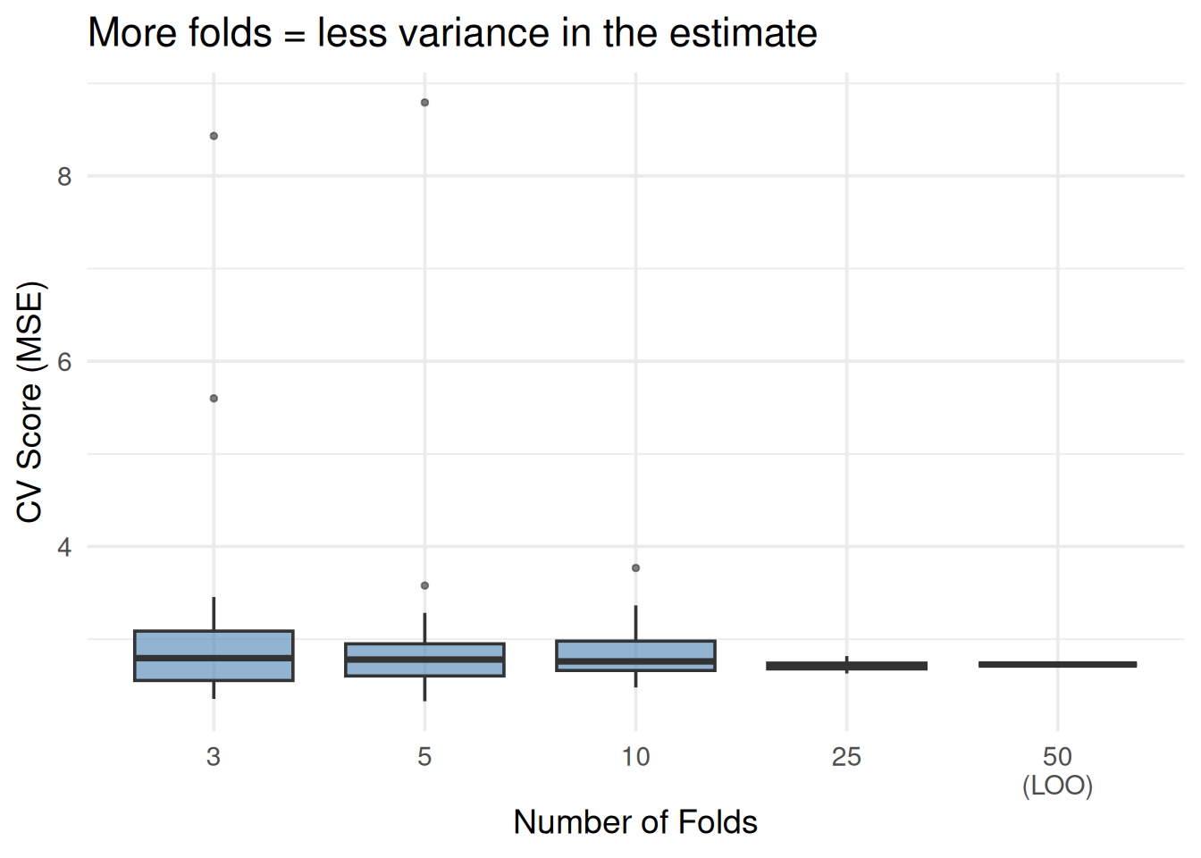
Figure 6: More folds = more stable estimate, but diminishing returns past 10

Rule of thumb for this guide: Use 5-fold or 10-fold. These are the standard choices and almost always sufficient.

5. What Cross-Validation Is Actually Used For

Cross-validation answers two questions:

Question 1: How good is this model?

“What accuracy will my SVM get on new data?” → Train with CV, report the average score.

Question 2: Which parameter value is best?

This is the primary use in this guide: choosing hyperparameters.

What \(k\) should I use in KNN?
What \(C\) should I use in SVM?
How many components in PCA?
Which variables in regression?

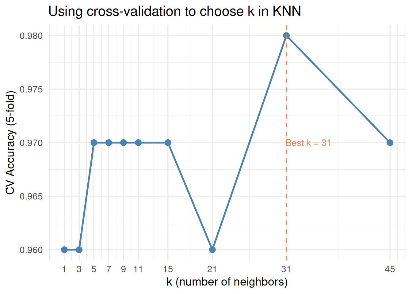
library(class)
set.seed(42)

# Generate classification data
df_class <- data.frame(
  x1 = c(rnorm(50, 2, 1), rnorm(50, 4.5, 1)),
  x2 = c(rnorm(50, 2, 1), rnorm(50, 4.5, 1)),
  group = factor(rep(c("A", "B"), each = 50))
)

# 5-fold CV for different k values
k_values <- c(1, 3, 5, 7, 9, 11, 15, 21, 31, 45)
n_obs <- nrow(df_class)
folds <- sample(rep(1:5, length.out = n_obs))

cv_results <- sapply(k_values, function(k_nn) {
  fold_acc <- sapply(1:5, function(f) {
    train <- df_class[folds != f, ]
    test <- df_class[folds == f, ]
    pred <- knn(train[, 1:2], test[, 1:2], train$group, k = k_nn)
    mean(pred == test$group)
  })
  mean(fold_acc)
})

best_k <- k_values[which.max(cv_results)]

ggplot(data.frame(k = k_values, accuracy = cv_results), aes(k, accuracy)) +
  geom_line(linewidth = 1, color = "steelblue") +
  geom_point(size = 3, color = "steelblue") +
  geom_vline(xintercept = best_k, linetype = "dashed", color = "coral") +
  annotate("text", x = best_k + 3, y = min(cv_results) + 0.01,
           label = paste0("Best k = ", best_k), color = "coral", size = 4) +
  scale_x_continuous(breaks = k_values) +
  theme_minimal(base_size = 14) +
  labs(x = "k (number of neighbors)", y = "CV Accuracy (5-fold)",
       title = "Using cross-validation to choose k in KNN")

Figure 7: Cross-validation finds the best k for KNN by testing each value

library(e1071)


Attaching package: 'e1071'

The following object is masked from 'package:ggplot2':

    element

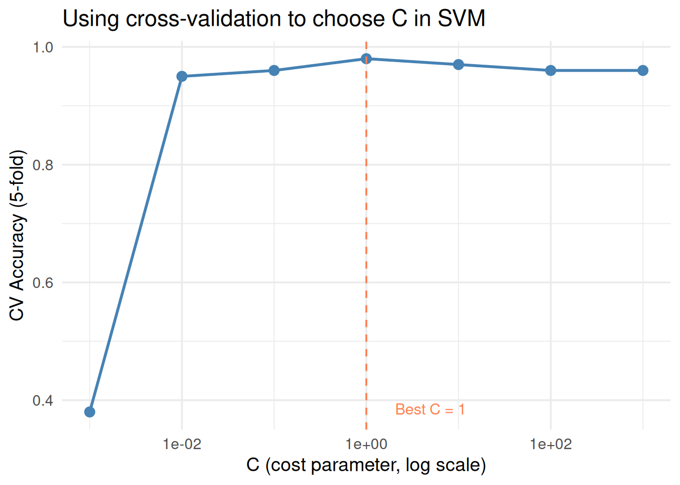
c_values <- c(0.001, 0.01, 0.1, 1, 10, 100, 1000)

cv_svm <- sapply(c_values, function(C) {
  fold_acc <- sapply(1:5, function(f) {
    train <- df_class[folds != f, ]
    test <- df_class[folds == f, ]
    fit <- svm(group ~ x1 + x2, data = train, kernel = "linear", cost = C)
    pred <- predict(fit, test)
    mean(pred == test$group)
  })
  mean(fold_acc)
})

best_c <- c_values[which.max(cv_svm)]

ggplot(data.frame(C = c_values, accuracy = cv_svm), aes(C, accuracy)) +
  geom_line(linewidth = 1, color = "steelblue") +
  geom_point(size = 3, color = "steelblue") +
  geom_vline(xintercept = best_c, linetype = "dashed", color = "coral") +
  annotate("text", x = best_c * 5, y = min(cv_svm) + 0.005,
           label = paste0("Best C = ", best_c), color = "coral", size = 4) +
  scale_x_log10() +
  theme_minimal(base_size = 14) +
  labs(x = "C (cost parameter, log scale)", y = "CV Accuracy (5-fold)",
       title = "Using cross-validation to choose C in SVM")

Figure 8: Same idea for SVM: cross-validate over different C values

6. The Train / Validate / Test Split

When you use CV to tune parameters, the CV folds become your validation set. You still need a separate test set that was never part of any tuning.

┌──────────────────────────────────────────────────────────┐
│  ALL DATA                                                │
│                                                          │
│  ┌────────────────────────────────┐  ┌────────────────┐  │
│  │  Training + Validation (80%)   │  │  Test Set (20%) │  │
│  │                                │  │                 │  │
│  │  ← cross-validation happens    │  │  ← touched ONCE │  │
│  │    here to tune parameters     │  │    at the very  │  │
│  │                                │  │    end          │  │
│  └────────────────────────────────┘  └────────────────┘  │
└──────────────────────────────────────────────────────────┘

The workflow:

Set aside 20% as the test set (lock it away)
Use the remaining 80% for k-fold CV to choose parameters
Retrain the final model on all 80% with the best parameters
Evaluate once on the test set → this is your reported performance

Why? If you tune on test data, you’re indirectly fitting to it. The test set must be truly unseen.

# Simulate the full workflow
set.seed(42)

# Step 1: Hold out test set
test_idx <- sample(n_obs, round(0.2 * n_obs))
train_val <- df_class[-test_idx, ]
test_final <- df_class[test_idx, ]

# Step 2: CV on train_val to find best k
folds_tv <- sample(rep(1:5, length.out = nrow(train_val)))

cv_k <- sapply(k_values, function(k_nn) {
  fold_acc <- sapply(1:5, function(f) {
    tr <- train_val[folds_tv != f, ]
    va <- train_val[folds_tv == f, ]
    pred <- knn(tr[, 1:2], va[, 1:2], tr$group, k = k_nn)
    mean(pred == va$group)
  })
  mean(fold_acc)
})

best_k_final <- k_values[which.max(cv_k)]

# Step 3: Evaluate on test set with best k
test_pred <- knn(train_val[, 1:2], test_final[, 1:2], train_val$group, k = best_k_final)
test_acc <- mean(test_pred == test_final$group)

cat(sprintf("Best k from CV: %d\n", best_k_final))

Best k from CV: 5

cat(sprintf("CV accuracy (validation): %.1f%%\n", max(cv_k) * 100))

CV accuracy (validation): 97.5%

cat(sprintf("Final test accuracy: %.1f%%\n", test_acc * 100))

Final test accuracy: 100.0%

cat("\nIf these two numbers are close → model generalizes well")


If these two numbers are close → model generalizes well

cat("\nIf test << CV → you overfit during tuning (rare with proper CV)")


If test << CV → you overfit during tuning (rare with proper CV)

7. Common Mistakes (Common Pitfalls)

Trap 1: Testing on Training Data

“Our model achieves 98% accuracy!”

“On what data?”

“The training data.”

Meaningless. A model that memorizes gets 100% on training data.

Trap 2: Confusing Training Accuracy with Real Performance

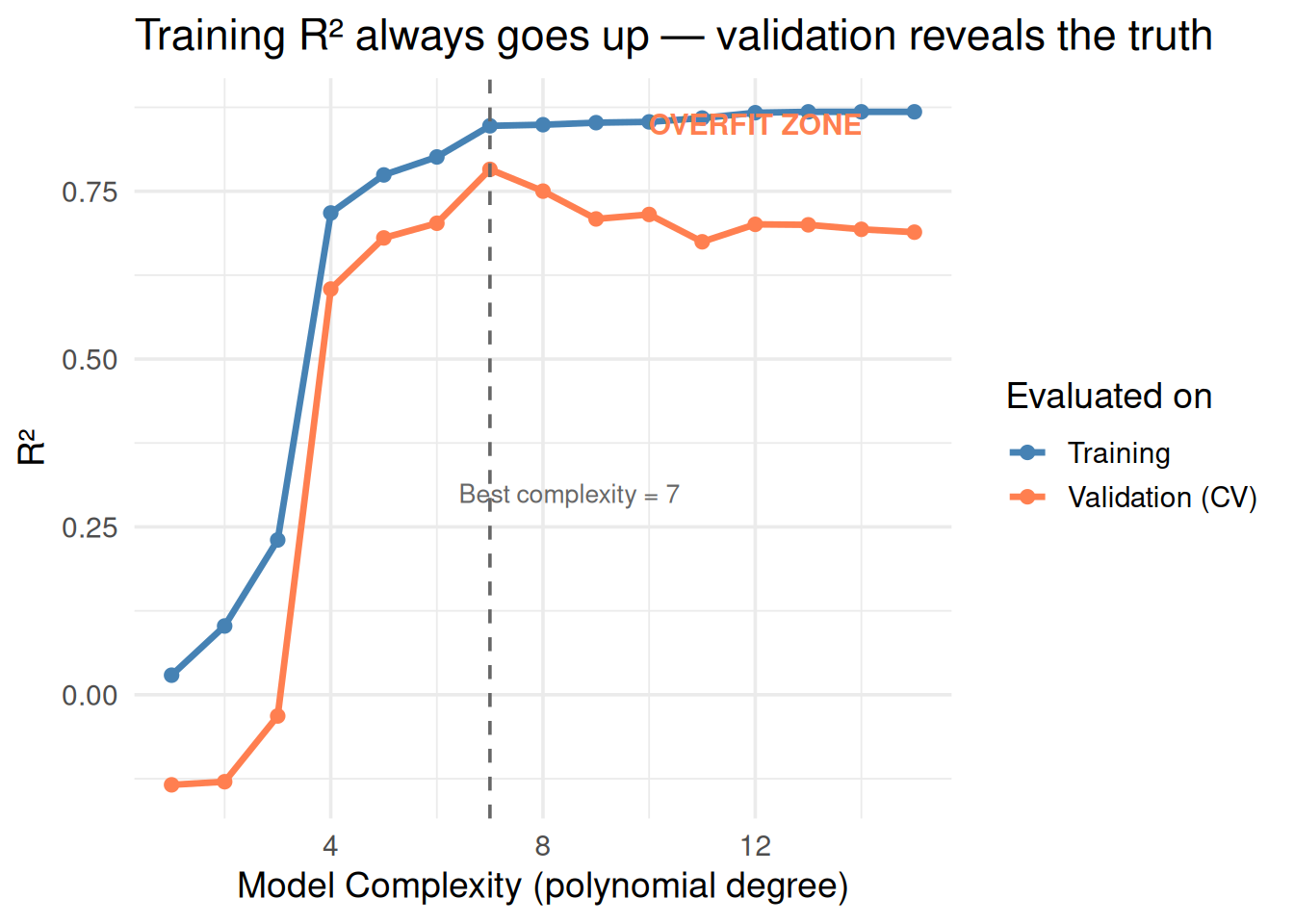
High training accuracy + low validation accuracy = overfitting.

The validation score is the one that matters.

# Show train vs validation accuracy across model complexity
complexities <- 1:15
train_acc <- numeric(15)
val_acc <- numeric(15)

set.seed(42)
folds_gap <- sample(rep(1:5, length.out = nrow(df_cv)))

for (d in complexities) {
  # Training accuracy (full data)
  fit <- lm(y ~ poly(x, d), data = df_cv)
  train_acc[d] <- 1 - mean(residuals(fit)^2) / var(df_cv$y)

  # CV accuracy
  fold_r2 <- sapply(1:5, function(f) {
    tr <- df_cv[folds_gap != f, ]
    te <- df_cv[folds_gap == f, ]
    if (nrow(tr) < d + 1) return(NA)
    fit_cv <- lm(y ~ poly(x, min(d, nrow(tr) - 2)), data = tr)
    pred <- predict(fit_cv, te)
    1 - mean((te$y - pred)^2) / var(te$y)
  })
  val_acc[d] <- mean(fold_r2, na.rm = TRUE)
}

gap_df <- data.frame(
  complexity = rep(complexities, 2),
  r_squared = c(train_acc, val_acc),
  set = rep(c("Training", "Validation (CV)"), each = 15)
)

ggplot(gap_df, aes(complexity, r_squared, color = set)) +
  geom_line(linewidth = 1.2) +
  geom_point(size = 2) +
  scale_color_manual(values = c("steelblue", "coral")) +
  geom_vline(xintercept = which.max(val_acc), linetype = "dashed", color = "gray40") +
  annotate("text", x = which.max(val_acc) + 1.5, y = 0.3,
           label = paste0("Best complexity = ", which.max(val_acc)),
           color = "gray40", size = 3.5) +
  annotate("text", x = 12, y = 0.85, label = "OVERFIT ZONE",
           color = "coral", size = 4, fontface = "bold") +
  theme_minimal(base_size = 14) +
  labs(x = "Model Complexity (polynomial degree)", y = "R²",
       color = "Evaluated on", title = "Training R² always goes up — validation reveals the truth")

Figure 9: The gap between training and validation accuracy reveals overfitting

Trap 3: Using Test Data to Tune Parameters

If you try 20 different values of \(k\) on the test set and pick the best one, you’ve fit to the test set. It’s no longer a fair evaluation.

Rule: Test set = used once, at the very end.

Trap 4: Not Enough Data in Each Fold

If \(n = 20\) and \(k = 10\), each test fold has only 2 points. That’s not enough for a reliable error estimate. Use fewer folds with small datasets.

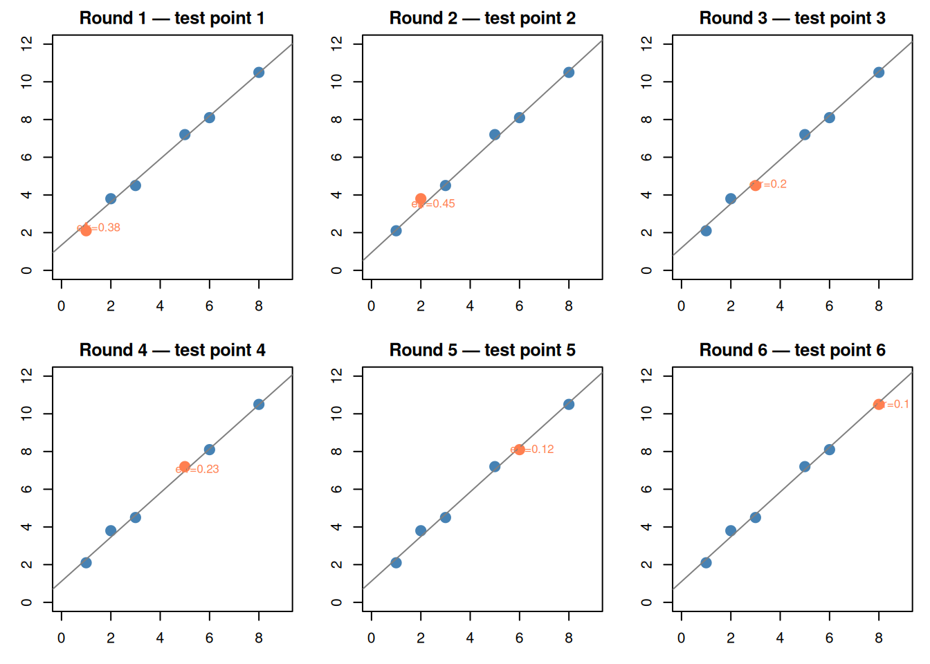
8. Special Case: Leave-One-Out Cross-Validation (LOOCV)

When \(k = n\) (number of folds = number of data points):

Each round: train on \(n-1\) points, test on 1 point
Repeat \(n\) times
Average all \(n\) errors

# Visual: highlight one point at a time
par(mfrow = c(2, 3), mar = c(3, 3, 2, 1))

set.seed(42)
small_df <- data.frame(
  x = c(1, 2, 3, 5, 6, 8),
  y = c(2.1, 3.8, 4.5, 7.2, 8.1, 10.5)
)

for (i in 1:6) {
  train <- small_df[-i, ]
  test <- small_df[i, ]
  fit <- lm(y ~ x, data = train)

  plot(small_df$x, small_df$y, pch = 19, cex = 1.5,
    col = ifelse(1:6 == i, "coral", "steelblue"),
    main = paste("Round", i, "— test point", i),
    xlab = "x", ylab = "y", xlim = c(0, 9), ylim = c(0, 12))
  abline(fit, col = "gray50")
  pred <- predict(fit, test)
  segments(test$x, test$y, test$x, pred, col = "coral", lwd = 2, lty = 2)
  text(test$x + 0.5, (test$y + pred) / 2,
       paste0("err=", round(abs(test$y - pred), 2)),
       col = "coral", cex = 0.8)
}
par(mfrow = c(1, 1))

Figure 10: LOOCV: each point gets a turn as the sole test point

LOOCV pros: Uses maximum training data (n-1 points each round). LOOCV cons: Runs \(n\) times (slow for large data), high variance.

When to use: Small datasets where every point matters.

9. Cheat Sheet: The Whole Story on One Page

CROSS-VALIDATION RECIPE
========================

1. PURPOSE: Estimate how well a model generalizes to unseen data

2. k-FOLD CV:
   - Split data into k equal folds
   - Each fold takes a turn as test set
   - Average the k scores
   - Standard choice: k = 5 or k = 10

3. THE FORMULA:
   CV(k) = (1/k) × Σ Errorᵢ

4. PRIMARY USE: Tune hyperparameters
   - KNN: which k (neighbors)?        → CV over k = 1,3,5,7,...
   - SVM: which C (cost)?             → CV over C = 0.01, 0.1, 1, 10,...
   - Regression: which variables?     → CV with different subsets
   - PCA: how many components?        → CV with 1, 2, 3, ... components

5. THREE-WAY SPLIT:
   Training (fit model) → Validation (tune params via CV) → Test (final eval)
   Test set: touched ONCE, at the very end

6. OVERFITTING DETECTION:
   Training accuracy >> Validation accuracy = OVERFIT
   Training accuracy ≈ Validation accuracy = GOOD

7. COMMON PITFALLS:
   - Never evaluate on training data
   - Never tune on test data
   - High training accuracy alone means NOTHING
   - The validation/CV score is what matters

10. Check Your Understanding

Test Yourself

Before moving on, try to answer these without scrolling up:

Why can’t you evaluate a model on its training data?
What does k-fold cross-validation do, step by step?
What’s the difference between the validation set and the test set?
How do you use cross-validation to choose \(k\) in KNN?
You build a model that gets 95% training accuracy and 62% validation accuracy. What’s happening? What would you do?
Why is leave-one-out CV sometimes worse than 10-fold, despite using more training data per round?
A classmate says “I tried 50 different models on the test set and picked the best one.” What’s wrong with this?