MCAR / MAR / MNAR, listwise deletion, indicators, and three imputation strategies
The Fiction in Clean Data
Most introductory examples treat a dataset as if every row is complete and every value is right. Real datasets never are. Sensors fail, forms get skipped, wireless signals drop, and high-income survey respondents leave the “income” field blank. The question is not whether you’ll have missing data — it’s what kind of missingness, and what to do about it.
Tip
Rule of thumb: before touching any imputation method, ask why the data is missing. The fix depends entirely on the cause.
Three Missingness Regimes
Formal acronyms are not always used, but the distinction is crucial:
Acronym
What it means
Example
MCAR (Missing Completely At Random)
Missingness unrelated to any variable
Sensor glitched for an hour; transmission dropped a packet
MAR (Missing At Random)
Missingness depends on observed variables
Men skip the “weight” field more often than women (depends on gender, which we have)
MNAR (Missing Not At Random)
Missingness depends on the unobserved value itself
High-income respondents skip the income field; date-of-death missing for living patients (censoring)
Why it matters: discarding rows is safe under MCAR, risky under MAR, and dangerous under MNAR. Let’s see the bias in action.
set.seed(2026)n <-1000age <-runif(n, 25, 65)job_yrs <-runif(n, 0, 40)# True income: depends on age and years of experienceincome <-20000+1500* age +800* job_yrs +rnorm(n, 0, 10000)dat <-data.frame(age, job_yrs, income)head(dat)
We have the truth. Now let’s hide some of it three different ways.
# MCAR: drop 20% of incomes completely at randommcar <- datmcar$income[sample(n, 200)] <-NA# MAR: older people skip more often (missingness depends on age, which we observe)p_miss_mar <-plogis(-5+0.1* dat$age)mar <- datmar$income[as.logical(rbinom(n, 1, p_miss_mar))] <-NA# MNAR: high-income people skip more often (missingness depends on income itself)p_miss_mnar <-plogis(-6+0.00008* dat$income)mnar <- datmnar$income[as.logical(rbinom(n, 1, p_miss_mnar))] <-NAmean_true <-mean(dat$income)mean_mcar <-mean(mcar$income, na.rm =TRUE)mean_mar <-mean(mar$income, na.rm =TRUE)mean_mnar <-mean(mnar$income, na.rm =TRUE)round(c(True = mean_true, MCAR = mean_mcar, MAR = mean_mar, MNAR = mean_mnar))
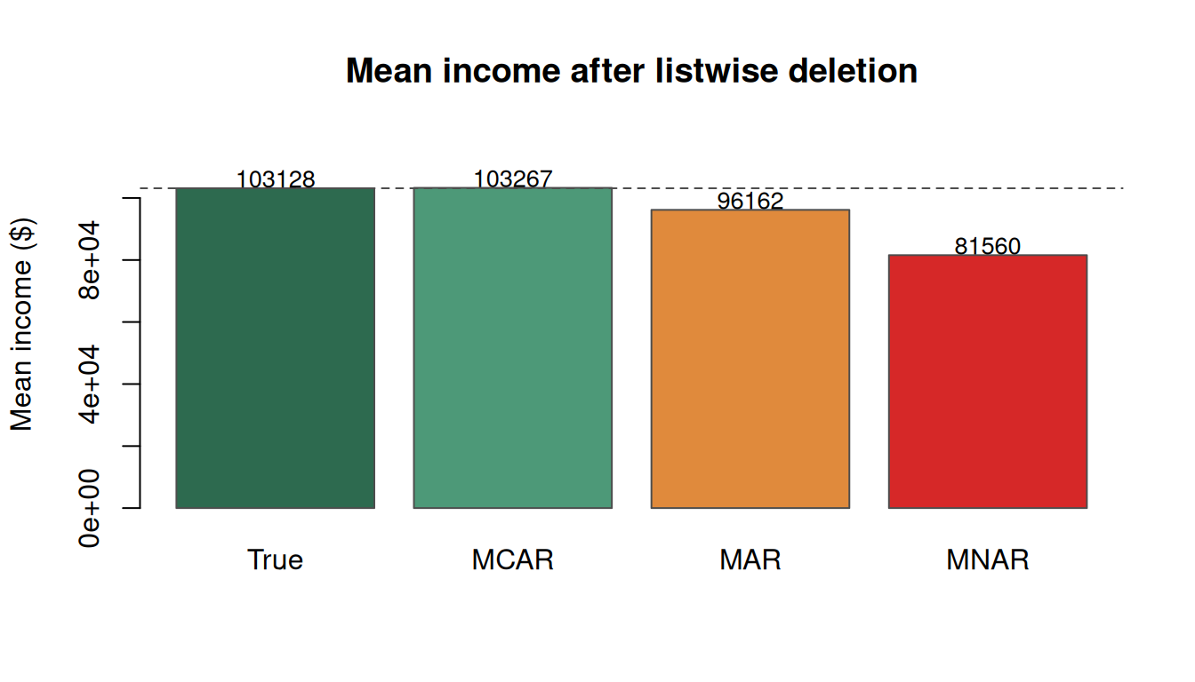
  True   MCAR    MAR   MNAR
103128 103267  96162  81560
MCAR barely shifts the mean (noise). MAR is only a modest shift because the observed variable (age) has a weak link to income. MNAR noticeably biases the mean downward because the highest-income values are the ones most likely to be missing.
Figure 1: Listwise-deletion bias by missingness regime. MCAR is safe; MNAR is the dangerous case.
Warning
Common pitfall: students love to assume missing data is random and “just drop the rows.” Discarding rows is only safe under MCAR. Under MNAR (the most common real-world case), your model becomes biased and you won’t know unless you specifically look.
Strategy 1 — Throw the Data Points Away
The simplest option is also the most dangerous. Do use listwise deletion when:
You’ve established the missingness is MCAR (or close to it), AND
The data loss is small enough that you still have adequate sample size.
Don’t use it when missingness is driven by the value you care about.
# Listwise deletion is just na.omit in Rcomplete_cases_mnar <-na.omit(mnar)cat("Original rows: ", nrow(mnar), "\n")
cat("Biased mean income: ", round(mean(complete_cases_mnar$income)), "\n")
Biased mean income: 81560
Strategy 2 — Add a “Missing” Indicator (and Interact It)
Instead of discarding, encode “this value is missing” as part of the model. For a categorical variable, just add a new level. For a numeric variable, the move is:
Set the missing values to 0 (or some placeholder).
Add a binary indicator is_missing.
Crucially: interact the indicator with every other predictor.
Step 3 is what makes this work. Without the interactions, the coefficients on the other variables get pulled in weird directions to compensate. With them, you’re effectively fitting two parallel models — one for rows with complete data, one for rows where this variable is missing — a “tree with one branch.”
# Start with the MAR datasetmar_ind <- marmar_ind$income_missing <-as.integer(is.na(mar_ind$income))mar_ind$income[is.na(mar_ind$income)] <-0# Without interactions — income coefficient gets contaminated by the zerosfit_bad <-lm(job_yrs ~ age + income + income_missing, data = mar_ind)# With interactions — effectively two modelsfit_good <-lm(job_yrs ~ age + income + income_missing + income:income_missing + age:income_missing,data = mar_ind)summary(fit_good)$coefficients |>round(4)
                   Estimate Std. Error  t value Pr(>|t|)
(Intercept)         -0.6077     1.9731  -0.3080   0.7581
age                 -0.8883     0.0581 -15.2880   0.0000
income               0.0006     0.0000  19.3068   0.0000
income_missing      20.4973     3.2655   6.2770   0.0000
age:income_missing   0.8828     0.0763  11.5738   0.0000
Note
Why interact with every other variable? Because the missing-indicator alone only shifts the intercept. To let the model respond differently to the other predictors when income is missing — which is what you actually want when missingness correlates with other features — you need the interactions.
Strategy 3 — Imputation (Three Flavors)
Imputation means estimating the missing values and filling them in. The three methods covered here trade off simplicity vs realism.
3a. Mean / Median / Mode Imputation
Simplest possible: replace each missing value with the mean (numeric), median (numeric, robust to skew), or mode (categorical).
cat("Mean-imputed mean income:", round(mean(imputed_mean$income)), "\n")
Mean-imputed mean income: 81560
Mean imputation preserves the mean of the imputed column but collapses all variance in the missing subset to zero, which distorts correlations and downstream models.
3b. Predictive Model Imputation (Regression)
Build a regression model on the rows without missing data that predicts the missing factor from the other factors. Use it to impute.
# Fit a model on the complete rowscomplete_rows <- mnar[!is.na(mnar$income), ]missing_rows <- mnar[is.na(mnar$income), ]impute_model <-lm(income ~ age + job_yrs, data = complete_rows)# Predict for the missing rowspredicted_income <-predict(impute_model, newdata = missing_rows)imputed_reg <- mnarimputed_reg$income[is.na(imputed_reg$income)] <- predicted_incomecat("Mean of imputed incomes (regression):", round(mean(predicted_income)), "\n")
This usually gives a better individual estimate than the global mean, but it still collapses legitimate variation — every 45-year-old with 15 years on the job gets the same predicted income, even though in the real population their incomes span a range.
3c. Regression + Perturbation
Fix the variance-collapse problem by adding random noise calibrated to the regression residual standard error:
# Residual standard error from the imputation modelres_sd <-summary(impute_model)$sigmaset.seed(2026)perturbed <- predicted_income +rnorm(length(predicted_income), 0, res_sd)imputed_pert <- mnarimputed_pert$income[is.na(imputed_pert$income)] <- perturbedcat("Regression-only SD in imputed values: ", round(sd(predicted_income)), "\n")
Regression-only SD in imputed values: 16727
cat("Regression+perturbation SD in imputed vals:", round(sd(perturbed)), "\n")
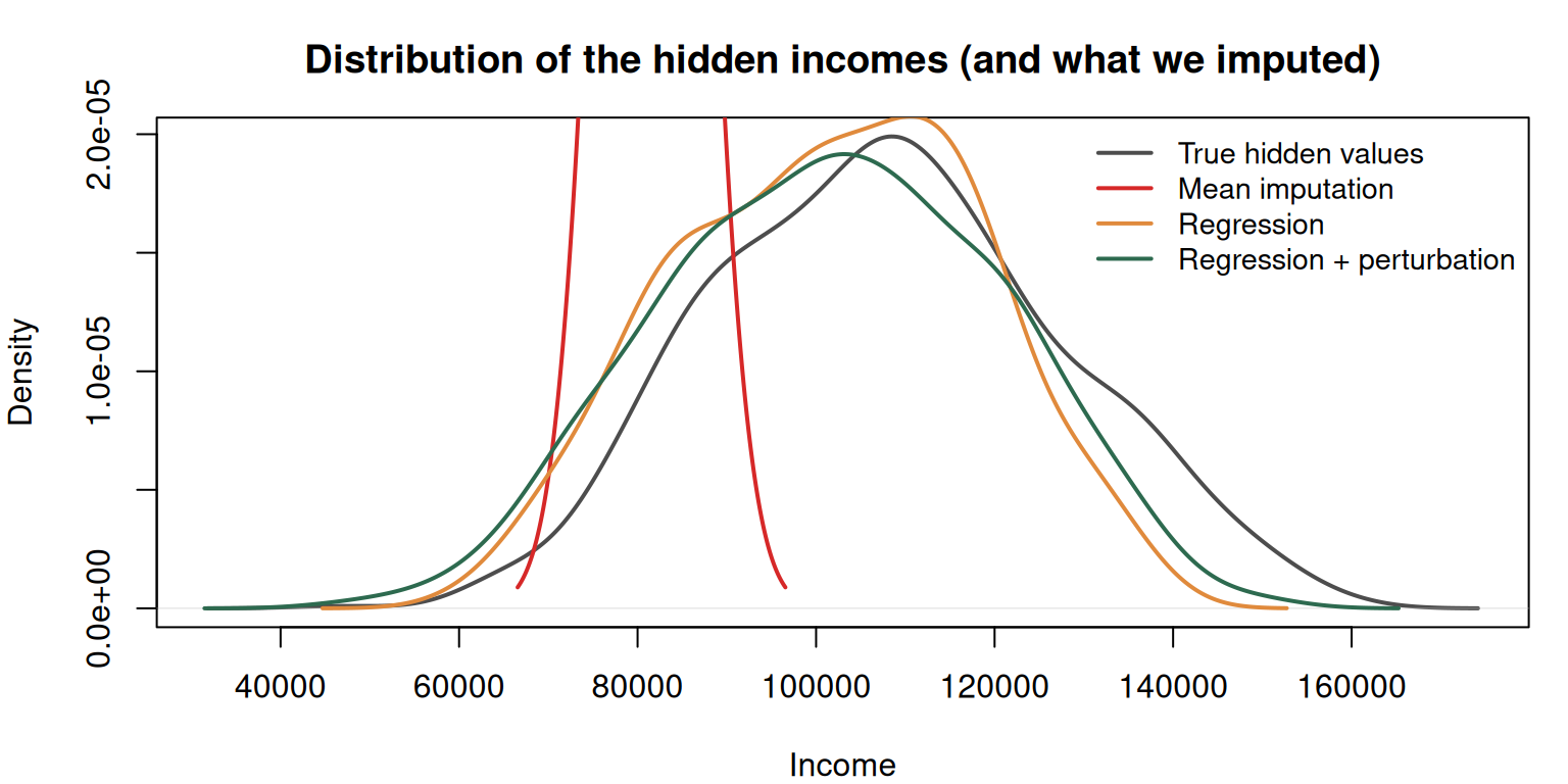
The perturbation looks like it makes each individual estimate worse (adding noise), but it preserves the spread of the imputed values. When variance matters downstream, this matters.
Figure 2: Three imputation strategies compared against the true distribution. Mean imputation collapses to a spike; regression collapses to a narrow band; perturbation restores the spread.
The 5% Rule
Tip
Rule of thumb: don’t impute more than about 5% of any single factor. Past that, switch to the indicator-plus-interaction approach from Strategy 2.
Why? Because imputation introduces error, and adding that error to more than a small slice of the data compounds. At that point you’re better off modeling the missingness explicitly rather than hiding it behind a guess.
Compounding Error — Honest Answer
You’re worried: “I’ve imputed values with error, now I’m feeding those into a model that also has error. How do I quantify the total error?”
The honest answer: there isn’t a clean way. Use a held-out test set to evaluate overall performance and accept that the test set itself probably has some missingness too.
Here’s the practical reframe: every dataset has errors — sensors drift, humans type wrong numbers, digital thermometers give different readings 10 seconds apart. The question is not “is my imputation perfect” but “is my imputation worse than the typical error already baked into the data?” Usually it isn’t.
Cheat Sheet
Situation
Best approach
Missingness tiny, clearly random
Listwise deletion (na.omit)
Missingness correlated with other variables
Indicator + interactions (Strategy 2)
Missingness correlated with the missing variable itself
Indicator + interactions (Strategy 2). Do NOT drop rows.
Small amount (<5%), value-dependent
Regression imputation, with perturbation if variance matters
>5% missing in one factor
Indicator approach, not imputation
Warning
Common pitfalls recap:
Listwise delete is not “safe default.” It’s only safe under MCAR.
Mean imputation is the easiest to do, the easiest to critique. Kills variance in the imputed subset.
Regression imputation needs perturbation if variance or correlations matter downstream.
The 5% rule kicks in before you notice it kicking in. Always check proportion missing per factor before choosing a strategy.
Indicator without interactions doesn’t split the model — it only shifts the intercept.