Design of Experiments: Collecting Data With Purpose

A/B testing, factorial designs, and multi-armed bandits

The Problem: You Don’t Have Data Yet

Most of this guide assumes data already exists. DOE flips that assumption: you need to design the data collection itself. When getting the full dataset isn’t possible or would take too long, you must decide what to test, how many tests to run, and how to structure the tests to get useful answers efficiently.

When DOE matters:

Choosing between banner ad designs (which gets more clicks?)
An online retailer deciding what products to suggest
Political polls — surveying only 600 people but needing representative coverage across demographics
Comparing medical treatments, agricultural methods, startup strategies

Comparison, Control, and Blocking

Before any specific method, two foundational concepts:

Comparison and Control

To determine whether red cars sell for more than blue cars, you must control for other factors. Comparing two-year-old red Porsches to ten-year-old blue family cars conflates color with age and car type. You need groups that are comparable in all dimensions except the one you’re testing.

Blocking Factors

A blocking factor is something that could create variation in your results. Car type (sports car vs. family car) is a blocking factor — sports cars are more likely to be red. By analyzing red sports cars separately from red family cars, you reduce variance in your estimates because you’ve accounted for one source of variation.

A/B Testing

The simplest DOE method: compare two alternatives by randomly assigning test subjects and measuring outcomes.

How It Works

Randomly show Ad A or Ad B to the first 2,000 visitors
Track clicks (binomial data)
Run a hypothesis test

# Banner ad A/B test results
clicks_A <- 46;  shown_A <- 1003
clicks_B <- 97;  shown_B <- 997

# Two-proportion z-test
result <- prop.test(c(clicks_A, clicks_B), c(shown_A, shown_B))

cat("Ad A click rate:", round(clicks_A / shown_A * 100, 1), "%\n")

Ad A click rate: 4.6 %

cat("Ad B click rate:", round(clicks_B / shown_B * 100, 1), "%\n")

Ad B click rate: 9.7 %

cat("p-value:", format.pval(result$p.value, digits = 3), "\n")

p-value: 1.21e-05

cat("Conclusion:", ifelse(result$p.value < 0.05,
    "Statistically significant difference — use Ad B",
    "No significant difference — either ad is fine"), "\n")

Conclusion: Statistically significant difference — use Ad B

Three Requirements

Requirement	Why It Matters
Enough data collected quickly	The answer must arrive in time to be useful
Representative sample	Results from one population may not apply to another
Test is small vs. total population	If you expect 2,500 views and test 2,000, only 500 remain to benefit

Key nuance: “No significant difference” is also a useful answer — it means you can choose either alternative based on other criteria (cost, aesthetics, etc.).

Factorial Designs

When you have multiple factors to test, not just two alternatives.

Full Factorial

Test every combination of factor levels:

Factor	Choices
Font	Arial, Roboto
Wording	“MS in Analytics”, “Analytics Masters”
Background	Gold, White

\(2 \times 2 \times 2 = 8\) combinations. Run all 8, then use ANOVA (Analysis of Variance) to decompose how much each factor contributes.

The Scaling Problem

Seven factors with three choices each: \(3^7 = 2{,}187\) combinations. That’s almost always too many to test.

Fractional Factorial

Test a carefully chosen subset of combinations. The subset must be balanced:

Each choice appears the same number of times
Each pair of choices appears the same number of times

This preserves the ability to estimate main effects without testing every combination.

Regression Approach

If factors are believed to be independent, use regression with categorical variables to estimate each factor’s effect from the subset. But watch out for interactions:

The Interaction Trap

A white font and a white background might each test well individually — but a white font on a white background would be unreadable. When factors interact, you need interaction terms in your regression, and you may need to test those specific combinations.

Multi-Armed Bandits

The Problem with Fixed Testing

With 10 alternatives tested 1,000 times each, you show the best ad only 1,000 times but show suboptimal ads 9,000 times. Every trial spent on a bad alternative is lost value.

Exploration vs. Exploitation

Strategy	Focus	Risk
Exploration	Getting more information (which is truly best?)	Wastes value on bad options
Exploitation	Using the apparent best option now	Might miss a better option

The multi-armed bandit algorithm balances both simultaneously.

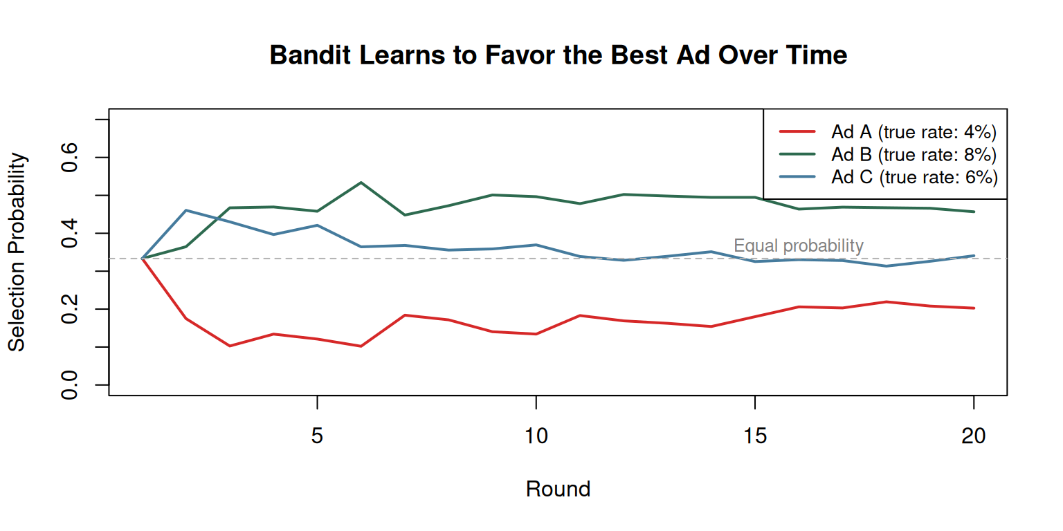
The Algorithm

set.seed(42)

# True click probabilities (unknown to the algorithm)
true_probs <- c(0.04, 0.08, 0.06)  # Ad A, B, C
K <- length(true_probs)
n_rounds <- 20
batch_size <- 50

# Track results
successes <- rep(0, K)
trials <- rep(0, K)
prob_history <- matrix(NA, nrow = n_rounds, ncol = K)

for (round in 1:n_rounds) {
  # Calculate selection probabilities (Thompson sampling approximation)
  if (round == 1) {
    probs <- rep(1/K, K)
  } else {
    # Estimate probability of each being best (simplified)
    rates <- (successes + 1) / (trials + 2)  # Laplace smoothing
    probs <- rates / sum(rates)
  }
  prob_history[round, ] <- probs

  # Assign batch according to probabilities
  assignments <- sample(1:K, batch_size, replace = TRUE, prob = probs)

  # Simulate outcomes
  for (k in 1:K) {
    n_assigned <- sum(assignments == k)
    if (n_assigned > 0) {
      trials[k] <- trials[k] + n_assigned
      successes[k] <- successes[k] + rbinom(1, n_assigned, true_probs[k])
    }
  }
}

# Plot probability evolution
cols <- c("#d62828", "#2d6a4f", "#457b9d")
matplot(1:n_rounds, prob_history, type = "l", lwd = 2, lty = 1, col = cols,
        xlab = "Round", ylab = "Selection Probability",
        main = "Bandit Learns to Favor the Best Ad Over Time",
        ylim = c(0, 0.7))
legend("topright", legend = paste0("Ad ", LETTERS[1:K],
       " (true rate: ", true_probs * 100, "%)"),
       col = cols, lwd = 2, cex = 0.85, bg = "white")
abline(h = 1/K, col = "gray70", lty = 2)
text(n_rounds * 0.8, 1/K + 0.03, "Equal probability", col = "gray50", cex = 0.8)

Name Origin

“One-armed bandit” = a slot machine (one lever arm, calibrated so you lose money on average). “Multi-armed bandit” = choosing among multiple slot machines with unknown payouts.

Parameters to Tune

Parameter	Options
Batch size	How many tests between recalculations
Probability updates	Bayesian updates vs. observed distributions
Assignment rule	Based on probability of being best, or on expected value

Connecting the Methods

Method	When to Use	Number of Alternatives	Adaptive?
A/B Testing	Simple comparison, two options	2	No (fixed test)
Factorial Design	Understand factor contributions	Many combinations	No (fixed design)
Multi-Armed Bandit	Choose best while minimizing waste	Multiple	Yes (learns as it goes)

All three address the same core question: how do I collect data efficiently to make a good decision? They differ in complexity, the number of alternatives, and whether the algorithm adapts during testing.

Common Pitfalls

Common Misconceptions

A/B testing requires a REPRESENTATIVE sample — results from college students may not apply to retirees. Sample must match the target population.
A/B testing also requires enough REMAINING population — if your test uses most of the population, there’s nobody left to benefit from the answer.
Full factorial tests ALL combinations — don’t confuse with fractional factorial, which tests a balanced subset.
Fractional factorial must be BALANCED — not any random subset of combinations works. Each choice and pair of choices must appear equally often.
Multi-armed bandits beat fixed testing — they learn faster AND earn more value during the learning process.
DOE happens BEFORE data collection — it’s about designing what data to collect, not analyzing data you already have.
Interaction terms can invalidate independence assumptions — the regression approach in factorial designs assumes factors don’t interact unless interaction terms are included.