CART From Scratch: Decision Trees That Think in If-Then Rules
The most interpretable model in machine learning
1. The Problem: Explain Your Decision
You’ve learned models that are powerful but hard to explain:
SVM: “the hyperplane with maximum margin decided…” (glazed eyes)
KNN: “the 5 nearest neighbors voted…” (what neighbors?)
Regression: “the weighted sum of 12 coefficients…” (too many numbers)
Sometimes you need a model that a non-technical person can read and follow. A loan officer. A doctor. A manager who asks “why did the model say no?”
CART gives you if-then rules that anyone can understand:
IF income > $50K AND credit_score > 700
  → APPROVE
ELSE IF income > $50K AND credit_score ≤ 700
  → REVIEW
ELSE
  → DENY
That’s a decision tree.
2. How CART Works: Splitting the Data
CART builds a tree by repeatedly splitting the data on the feature that best separates the groups.
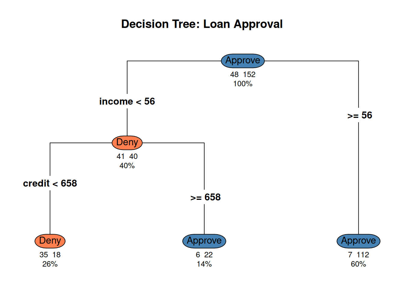
library(ggplot2)library(rpart)library(rpart.plot)set.seed(42)n <-200income <-runif(n, 20, 100)credit <-runif(n, 400, 850)# Decision rule: approve if income > 50 AND credit > 650 (with noise)prob_approve <-plogis(-5+0.06* income +0.005* credit)approved <-rbinom(n, 1, prob_approve)df <-data.frame(income = income,credit = credit,decision =factor(approved, labels =c("Deny", "Approve")))# Fit a treetree <-rpart(decision ~ income + credit, data = df, method ="class",control =rpart.control(maxdepth =3, cp =0.02))rpart.plot(tree, type =4, extra =101, under =TRUE,main ="Decision Tree: Loan Approval",box.palette =c("coral", "steelblue"))
Figure 1: CART splits the space into rectangles using if-then rules
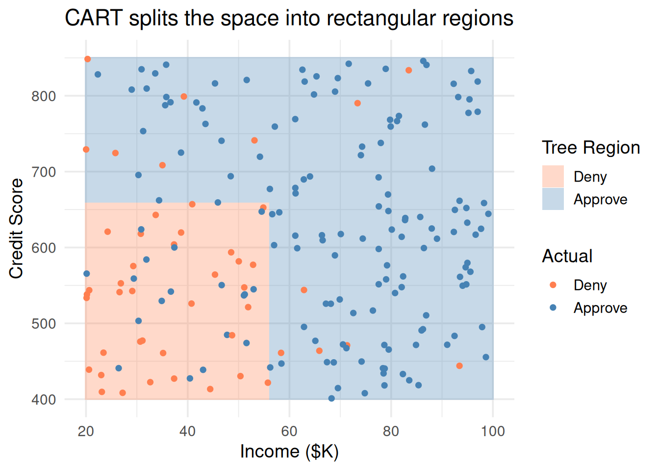
# Show the rectangular regionsgrid <-expand.grid(income =seq(20, 100, length.out =200),credit =seq(400, 850, length.out =200))grid$pred <-predict(tree, grid, type ="class")ggplot() +geom_tile(data = grid, aes(income, credit, fill = pred), alpha =0.3) +geom_point(data = df, aes(income, credit, color = decision), size =1.5) +scale_fill_manual(values =c("coral", "steelblue")) +scale_color_manual(values =c("coral", "steelblue")) +theme_minimal(base_size =14) +labs(x ="Income ($K)", y ="Credit Score",fill ="Tree Region", color ="Actual",title ="CART splits the space into rectangular regions")
Figure 2: Each split creates a rectangular region — the tree carves up the feature space
Compare this to SVM (which draws a single line/curve) or KNN (which draws irregular boundaries). CART always makes axis-aligned rectangular splits.
3. The Splitting Rule: How CART Chooses Where to Cut
At each step, CART asks: “which feature and which split point best separates the classes?”
For Classification: Gini Impurity
\[\text{Gini} = 1 - \sum_{k=1}^{K} p_k^2\]
where \(p_k\) is the proportion of class \(k\) in the node.
Gini Value
Meaning
0
Pure — all points belong to one class
0.5
Maximum impurity — 50/50 split (for 2 classes)
CART picks the split that creates the lowest weighted average Gini across the two child nodes.
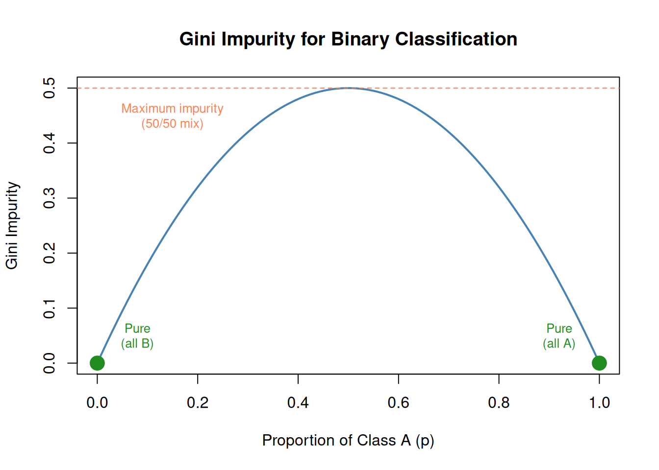
p <-seq(0, 1, length.out =100)gini <-2* p * (1- p) # simplified for 2 classes: 1 - p² - (1-p)²plot(p, gini, type ="l", lwd =2, col ="steelblue",main ="Gini Impurity for Binary Classification",xlab ="Proportion of Class A (p)", ylab ="Gini Impurity")abline(h =0.5, lty =2, col ="coral")text(0.15, 0.45, "Maximum impurity\n(50/50 mix)", col ="coral", cex =0.8)points(0, 0, pch =19, cex =2, col ="forestgreen")points(1, 0, pch =19, cex =2, col ="forestgreen")text(0.08, 0.05, "Pure\n(all B)", col ="forestgreen", cex =0.8)text(0.92, 0.05, "Pure\n(all A)", col ="forestgreen", cex =0.8)
Figure 3: Gini impurity: 0 = pure node, 0.5 = maximum mixed
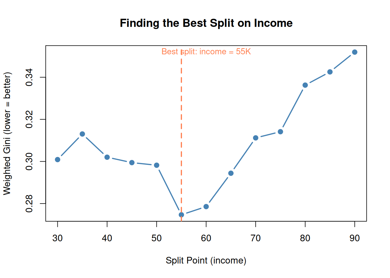
# Simple example: split on income at different pointssplit_points <-seq(30, 90, by =5)gini_scores <-sapply(split_points, function(sp) { left <- df$decision[df$income <= sp] right <- df$decision[df$income > sp] gini_left <-1-sum((table(left) /length(left))^2) gini_right <-1-sum((table(right) /length(right))^2)# Weighted average n_left <-length(left) n_right <-length(right) (n_left * gini_left + n_right * gini_right) / (n_left + n_right)})best_split <- split_points[which.min(gini_scores)]plot(split_points, gini_scores, type ="b", pch =19, col ="steelblue", lwd =2,main ="Finding the Best Split on Income",xlab ="Split Point (income)", ylab ="Weighted Gini (lower = better)")abline(v = best_split, col ="coral", lty =2, lwd =2)text(best_split +5, max(gini_scores),paste0("Best split: income = ", best_split, "K"),col ="coral", cex =0.9)
Figure 4: CART evaluates every possible split and picks the one with lowest total Gini
For Regression Trees: Sum of Squared Errors
When predicting a number instead of a class, CART minimizes SSE at each split — same objective as linear regression, but applied locally in each rectangle.
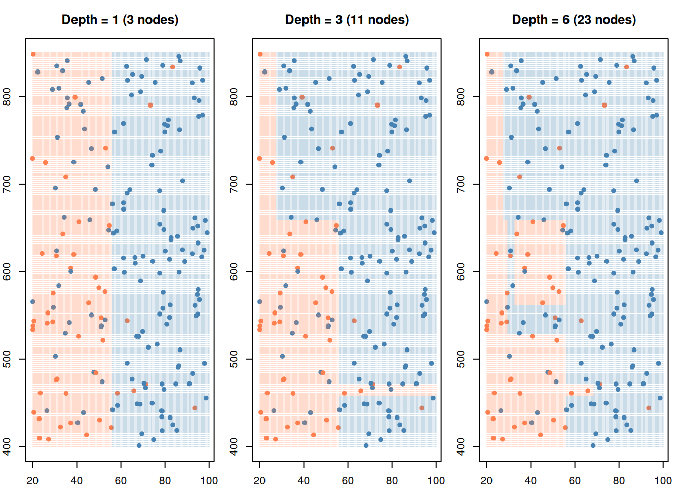
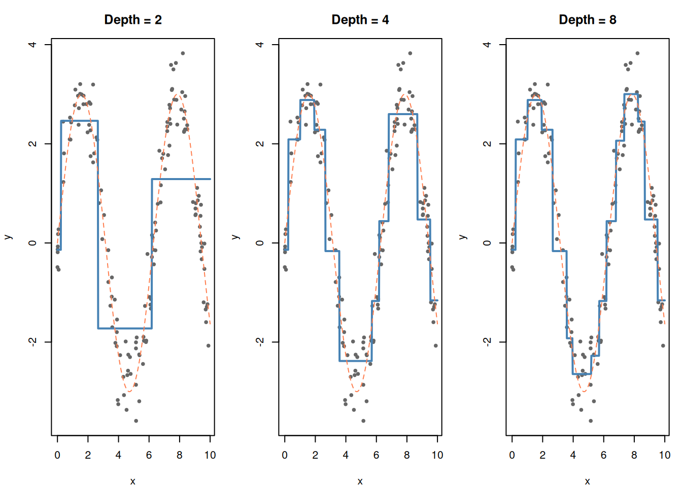
Figure 5: Deeper trees create more splits — from simple to complex
A deeper tree creates more rectangles — fitting the training data more closely. But there’s a problem…
5. The Overfitting Trap: Deep Trees Memorize
WarningDeep Trees Memorize
A tree with enough depth can perfectly classify every training point. But it’s just memorizing — it won’t work on new data.
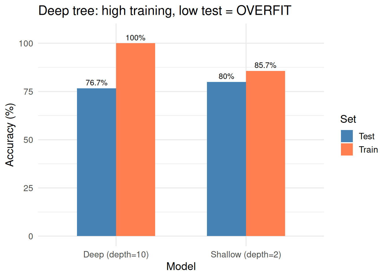
set.seed(42)# Split into train/testtrain_idx <-sample(n, round(0.7* n))train <- df[train_idx, ]test <- df[-train_idx, ]# Shallow treetree_shallow <-rpart(decision ~ income + credit, data = train, method ="class",control =rpart.control(maxdepth =2, cp =0.01))# Deep tree (overfit)tree_deep <-rpart(decision ~ income + credit, data = train, method ="class",control =rpart.control(maxdepth =10, cp =0.001, minsplit =2))# Accuraciestrain_acc_shallow <-mean(predict(tree_shallow, train, type ="class") == train$decision)test_acc_shallow <-mean(predict(tree_shallow, test, type ="class") == test$decision)train_acc_deep <-mean(predict(tree_deep, train, type ="class") == train$decision)test_acc_deep <-mean(predict(tree_deep, test, type ="class") == test$decision)results <-data.frame(Model =rep(c("Shallow (depth=2)", "Deep (depth=10)"), each =2),Set =rep(c("Train", "Test"), 2),Accuracy =c(train_acc_shallow, test_acc_shallow, train_acc_deep, test_acc_deep))ggplot(results, aes(Model, Accuracy *100, fill = Set)) +geom_col(position ="dodge", width =0.6) +scale_fill_manual(values =c("steelblue", "coral")) +geom_text(aes(label =paste0(round(Accuracy *100, 1), "%")),position =position_dodge(0.6), vjust =-0.5, size =3.5) +ylim(0, 105) +theme_minimal(base_size =14) +labs(y ="Accuracy (%)", title ="Deep tree: high training, low test = OVERFIT")
Figure 6: Deep tree: perfect on training data, terrible on new data
Signs of an overfit tree:
High training accuracy, low test accuracy
Many levels / many leaves
Some leaves have very few data points
Complex rules that don’t make intuitive sense
6. The Fix: Pruning
Pruning cuts back branches that don’t improve generalization. There are two strategies:
Strategy
How it works
Pre-pruning
Stop growing early (limit depth, minimum samples per leaf)
Post-pruning
Grow the full tree, then cut back branches that don’t help on validation data
# Grow a full treetree_full <-rpart(decision ~ income + credit, data = train, method ="class",control =rpart.control(cp =0.001, minsplit =2))# Find best CP via cross-validationprintcp(tree_full)
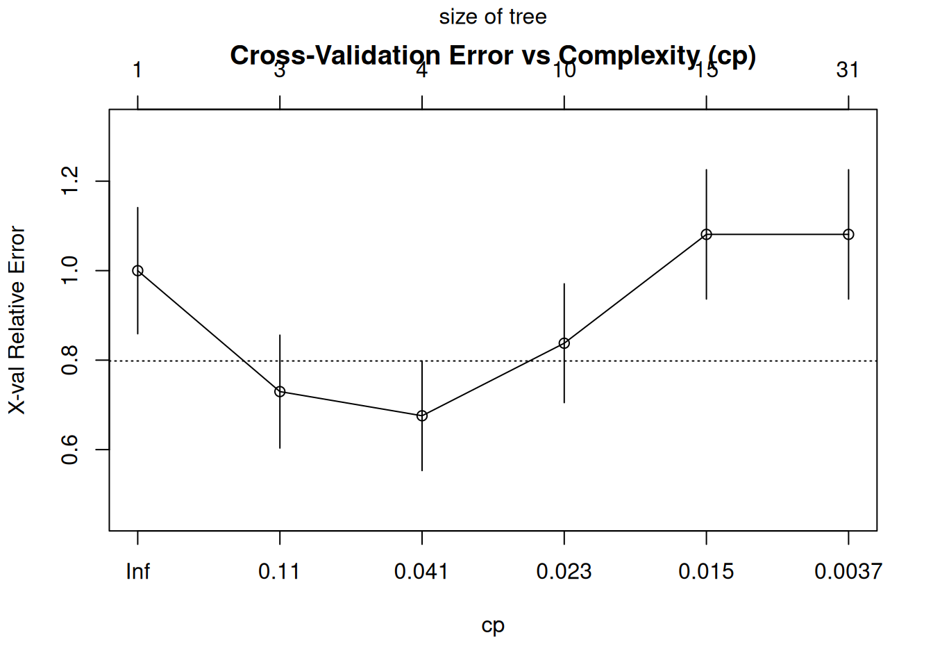
# Plot CP tableplotcp(tree_full, main ="Cross-Validation Error vs Complexity (cp)")
Figure 7: Pruning: grow a full tree, then trim branches that don’t help
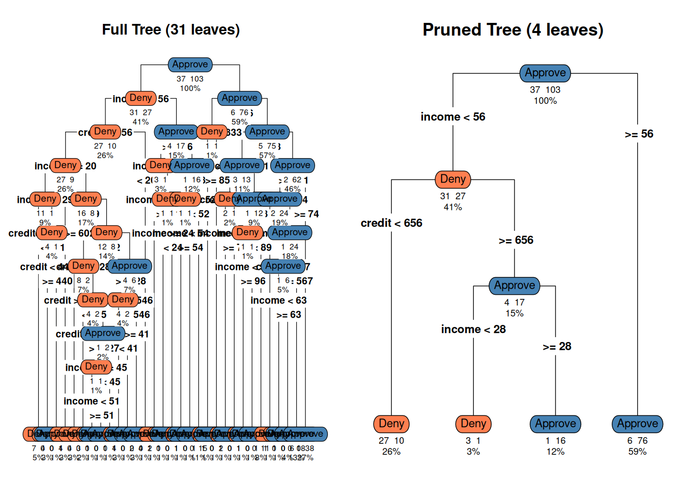
# Prune to optimal cpbest_cp <- tree_full$cptable[which.min(tree_full$cptable[, "xerror"]), "CP"]tree_pruned <-prune(tree_full, cp = best_cp)par(mfrow =c(1, 2), mar =c(2, 2, 3, 1))rpart.plot(tree_full, type =4, extra =101, under =TRUE,main =paste0("Full Tree (", sum(tree_full$frame$var =="<leaf>"), " leaves)"),box.palette =c("coral", "steelblue"), cex =0.6)
Warning: labs do not fit even at cex 0.15, there may be some overplotting
rpart.plot(tree_pruned, type =4, extra =101, under =TRUE,main =paste0("Pruned Tree (", sum(tree_pruned$frame$var =="<leaf>"), " leaves)"),box.palette =c("coral", "steelblue"), cex =0.7)par(mfrow =c(1, 1))# Compare test accuracyacc_full <-mean(predict(tree_full, test, type ="class") == test$decision)acc_pruned <-mean(predict(tree_pruned, test, type ="class") == test$decision)cat(sprintf("Full tree test accuracy: %.1f%%\n", acc_full *100))
Full tree test accuracy: 76.7%
cat(sprintf("Pruned tree test accuracy: %.1f%%\n", acc_pruned *100))
Pruned tree test accuracy: 80.0%
cat("Simpler tree often performs just as well (or better) on new data!")
Simpler tree often performs just as well (or better) on new data!
Figure 8: The pruned tree: simpler, more generalizable
7. CART for Regression
CART isn’t just for classification. It can predict continuous values too. Instead of majority vote in each leaf, it predicts the mean of the training points in that leaf.
set.seed(42)x_reg <-runif(150, 0, 10)y_reg <-sin(x_reg) *3+rnorm(150, 0, 0.5)df_reg <-data.frame(x = x_reg, y = y_reg)# Fit regression trees of different depthspar(mfrow =c(1, 3), mar =c(4, 4, 3, 1))for (depth inc(2, 4, 8)) { tree_reg <-rpart(y ~ x, data = df_reg,control =rpart.control(maxdepth = depth, cp =0.001)) x_grid <-data.frame(x =seq(0, 10, length.out =500)) x_grid$pred <-predict(tree_reg, x_grid)plot(df_reg$x, df_reg$y, pch =19, cex =0.6, col ="gray40",main =paste("Depth =", depth),xlab ="x", ylab ="y")lines(x_grid$x, x_grid$pred, col ="steelblue", lwd =2)lines(x_grid$x, sin(x_grid$x) *3, col ="coral", lty =2)}par(mfrow =c(1, 1))
Figure 9: Regression tree: predicts the average value in each rectangular region
Notice the staircase shape — regression trees make piecewise-constant predictions (flat steps). They approximate curves by breaking them into enough small rectangles.
8. CART vs Other Models
CART
SVM
KNN
Logistic Reg
Interpretable?
Yes — if-then rules
Moderate
No
Moderate (coefficients)
Handles non-linear?
Yes (inherently)
Yes (kernels)
Yes (inherently)
Only with transforms
Handles mixed types?
Yes (numeric + categorical)
Numeric only
Numeric only
Numeric only
Needs scaling?
No
Yes
Yes
Recommended
Overfitting risk
High (deep trees)
Moderate
High (small k)
Low
Feature selection?
Built in (top splits = most important)
No
No
Via p-values
CART’s unique advantages:
No scaling needed — splits are based on thresholds, not distances
Handles mixed data — categorical and numeric features together
Built-in feature importance — features used in top splits matter most
Human-readable — the only model a non-technical stakeholder can follow
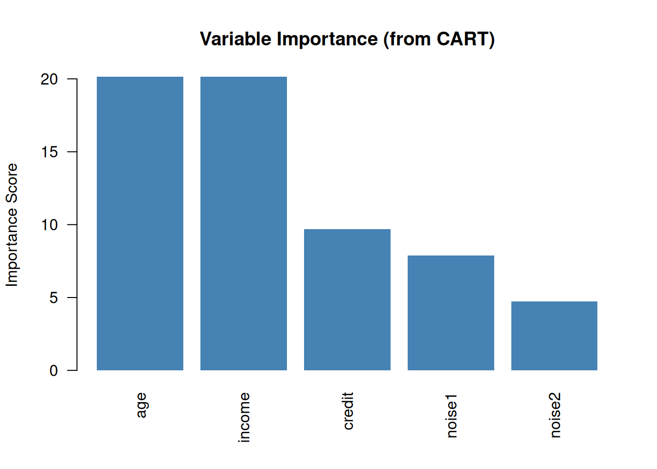
# Fit a tree with more featuresset.seed(42)df_imp <-data.frame(income = income,credit = credit,age =runif(n, 22, 70),noise1 =rnorm(n),noise2 =runif(n),decision = df$decision)tree_imp <-rpart(decision ~ ., data = df_imp, method ="class",control =rpart.control(maxdepth =4, cp =0.01))importance <- tree_imp$variable.importancebarplot(sort(importance, decreasing =TRUE),col ="steelblue", border =NA, las =2,main ="Variable Importance (from CART)",ylab ="Importance Score")
Figure 10: CART naturally tells you which features are most important
9. When to Use CART (Practice Scenarios)
Scenario
Use CART?
Why
“Need interpretable rules for a loan officer”
Yes
CART = human-readable if-then rules
“Explain to management why the model rejected an applicant”
Yes
Trace the tree path
“Classify with maximum accuracy on large dataset”
Maybe not
SVM often more accurate
“Features are a mix of numbers and categories”
Yes
CART handles both natively
“Predict a probability”
Logistic regression
CART outputs class, not calibrated probability
“Non-linear relationships, need simple explanation”
Yes
Splits naturally capture non-linearity
Connection to advanced models:
Random Forest = many CART trees averaged together (reduces overfitting)
Gradient Boosting = sequential CART trees correcting each other’s errors
These are the most powerful ML models in practice, and they’re all built from CART
10. Cheat Sheet: The Whole Story on One Page
CART (Decision Tree) RECIPE
=============================

1. ALGORITHM:
   - Pick the feature + split point with lowest Gini impurity (classification)
     or lowest SSE (regression)
   - Split the data into two groups
   - Repeat recursively on each group
   - Stop when a stopping criterion is met (depth, min samples, etc.)

2. SPLITTING CRITERIA:
   Classification: Gini = 1 - Σpₖ²    (0 = pure, 0.5 = max impurity)
   Regression:     SSE = Σ(yᵢ - ȳ)²   (minimize within each split)

3. OVERFITTING:
   Deep trees memorize → prune!
   Pre-pruning: limit depth, min samples per leaf
   Post-pruning: grow full tree, cut back branches (use cp / cross-validation)

4. UNIQUE ADVANTAGES:
   - Human-readable (if-then rules)
   - No scaling required
   - Handles mixed data (numeric + categorical)
   - Built-in feature importance
   - Non-linear without transforms

5. WEAKNESSES:
   - High overfitting risk without pruning
   - Axis-aligned splits only (rectangular boundaries)
   - Unstable: small data changes → very different tree

6. PRACTICE TIPS:
   "Interpretable model" → CART
   "Explain the decision" → CART
   "Perfect training accuracy" → overfit, prune it
   Building block for Random Forest and Boosting
11. Check Your Understanding
NoteTest Yourself
Before moving on, try to answer these without scrolling up:
Why is CART called the most “interpretable” model?
What is Gini impurity? What value means a pure node? A maximally mixed node?
How does CART decide where to split?
A decision tree gets 100% accuracy on training data. Is this good? What should you do?
What is pruning? Why is it necessary?
Name two advantages CART has over SVM.
Name two advantages SVM has over CART.
A manager says “I need to explain to the board why we denied this loan.” Which model would you recommend? Why?
How does a regression tree differ from a classification tree?
What are Random Forests and Gradient Boosting, and how do they relate to CART?