Advanced Topics: The Rapid Tour

Nonparametric tests, Bayesian shrinkage, neural nets, game theory, survival, and gradient boosting

A Fast Tour of Several Modeling Families

This is a greatest-hits tour of methods every analytics practitioner should recognize, even if each one could fill its own deep dive. The goal is not mastery in one sitting; it is vocabulary, intuition, and a working mental hook for where each method belongs.

This demo gives you one working R snippet per area so the names click into the concrete code they map to.

1. Nonparametric Tests

When you don’t know (or can’t assume) an underlying distribution, three go-to tests:

Test	Data	Question
McNemar’s test	Paired binary outcomes	Do two treatments differ?
Wilcoxon signed-rank	Paired or one-sample continuous	Is the median different?
Mann-Whitney U	Two independent samples	Are the distributions different?

McNemar’s test — paired binary outcomes

Two antibiotics tested against 50 bacterial strains each. For each strain, record whether A worked (1/0) and whether B worked (1/0).

set.seed(99)
n_strains <- 50
A_works <- rbinom(n_strains, 1, 0.55)
B_works <- rbinom(n_strains, 1, 0.80)

# McNemar ignores both-agree cells, tests the disagreement
contingency <- table(A_works, B_works)
contingency

       B_works
A_works  0  1
      0  4 17
      1  7 22

mcnemar.test(contingency, correct = FALSE)


    McNemar's Chi-squared test

data:  contingency
McNemar's chi-squared = 4.1667, df = 1, p-value = 0.04123

The test looks only at disagreement cells. If one treatment dominates the disagreements, the p-value is small.

Wilcoxon signed-rank — paired median comparison

set.seed(7)
before <- rnorm(30, mean = 100, sd = 12)
after  <- before - rnorm(30, mean = 4, sd = 6)   # slight improvement

wilcox.test(before, after, paired = TRUE)


    Wilcoxon signed rank exact test

data:  before and after
V = 416, p-value = 4.968e-05
alternative hypothesis: true location shift is not equal to 0

Mann-Whitney U — unpaired

group_a <- rnorm(40, mean = 50, sd = 10)
group_b <- rnorm(40, mean = 55, sd = 10)

wilcox.test(group_a, group_b, paired = FALSE)


    Wilcoxon rank sum exact test

data:  group_a and group_b
W = 411, p-value = 0.0001311
alternative hypothesis: true location shift is not equal to 0

Tip

Picking the right test: How many samples? If two, paired or unpaired? And what are you asking about (mean, median, success count)? That’s 80% of the decision.

2. Bayesian Modeling — Medical Test Gotcha

Bayes rule:

\[ P(A \mid B) = \frac{P(B \mid A) \cdot P(A)}{P(B)} \]

The classic medical test example: 98% sensitive, 8% false positive rate, 1% prevalence.

sensitivity <- 0.98    # P(+ | disease)
fpr         <- 0.08    # P(+ | no disease)
prevalence  <- 0.01

p_positive <- sensitivity * prevalence + fpr * (1 - prevalence)
p_disease_given_positive <- sensitivity * prevalence / p_positive

cat("P(positive test) =", round(p_positive, 4), "\n")

P(positive test) = 0.089

cat("P(disease | positive) =",
    round(p_disease_given_positive, 4),
    "(only about 11%!)\n")

P(disease | positive) = 0.1101 (only about 11%!)

Counter-intuitive: after a positive test, you still only have an ~11% chance of having the disease, because the large healthy population creates ~8× more false positives than the sick population creates true positives.

Empirical Bayes shrinkage — NCAA basketball

A sports analytics example: a 20-point home win is actually less than a 50% predictor of the same team winning on the road. Let’s see the shrinkage numbers.

# Parameters from historical NCAA data
H <- 4        # home-court advantage (points)
sigma <- 11   # SD of random game noise
tau <- 6      # SD of true team-strength differences

observed_margin <- 20
# Observed = H + M + noise, so "signal" = observed - H = 16 on top of home court

# Shrinkage: posterior mean of M given observation
# M | X ~ Normal(posterior_mean, posterior_var)
x_minus_h <- observed_margin - H
posterior_var  <- 1 / (1 / tau^2 + 1 / sigma^2)
posterior_mean <- posterior_var * (x_minus_h / sigma^2)

cat("Observed margin:             ", observed_margin, "\n")

Observed margin:              20

cat("  - home-court component:    ", H, "\n")

  - home-court component:     4

cat("  - posterior mean of M:     ", round(posterior_mean, 2), "\n")

  - posterior mean of M:      3.67

cat("  - attributed to randomness:",
    round(observed_margin - H - posterior_mean, 2), "\n")

  - attributed to randomness: 12.33

cat("P(home team is truly better) =",
    round(1 - pnorm(0, posterior_mean, sqrt(posterior_var)), 3), "\n")

P(home team is truly better) = 0.757

The model attributes ~4 points to home court, only ~3.5 to actual talent, and the rest to noise. That’s shrinkage in action.

3. Communities in Graphs — Louvain Sketch

Louvain maximizes modularity — a measure of how much more tightly nodes are connected within a community than you’d expect by random chance. Each round:

Start with every node in its own community.
Move each node to whichever neighbor community best increases modularity.
Repeat until stable.
Collapse each community into a super-node; go back to step 2.

We’ll hand-compute modularity for a tiny 6-node graph with two obvious communities.

# Adjacency matrix for two triangles connected by a single edge
A <- matrix(0, 6, 6)
# Triangle 1: nodes 1, 2, 3
A[1, 2] <- 1; A[2, 1] <- 1
A[1, 3] <- 1; A[3, 1] <- 1
A[2, 3] <- 1; A[3, 2] <- 1
# Triangle 2: nodes 4, 5, 6
A[4, 5] <- 1; A[5, 4] <- 1
A[4, 6] <- 1; A[6, 4] <- 1
A[5, 6] <- 1; A[6, 5] <- 1
# Bridge: 3-4
A[3, 4] <- 1; A[4, 3] <- 1

# Node weights (degree)
w <- rowSums(A)
# Total edge weight (undirected: sum(A) counts each edge twice)
W <- sum(A) / 2

modularity <- function(A, communities, w, W) {
  Q <- 0
  for (i in seq_along(communities)) {
    for (j in seq_along(communities)) {
      if (communities[i] == communities[j]) {
        Q <- Q + (A[i, j] - w[i] * w[j] / (2 * W))
      }
    }
  }
  Q / (2 * W)
}

# Two-community split (the "right" answer)
comm_good <- c(1, 1, 1, 2, 2, 2)
# Each-own community
comm_singleton <- 1:6
# One big community
comm_single <- rep(1, 6)

cat("Modularity (two communities):  ", round(modularity(A, comm_good, w, W), 3), "\n")

Modularity (two communities):   0.357

cat("Modularity (each own cluster): ", round(modularity(A, comm_singleton, w, W), 3), "\n")

Modularity (each own cluster):  -0.173

cat("Modularity (all one cluster):  ", round(modularity(A, comm_single, w, W), 3), "\n")

Modularity (all one cluster):   0

The two-community split maximizes modularity, which is the structural insight Louvain would climb to automatically.

4. Neural Networks — A Tiny Working Example

nnet ships with base R. Let’s train a 1-hidden-layer network on iris to classify species.

suppressMessages(library(nnet))

set.seed(1)

# Scale features
iris_scaled <- iris
iris_scaled[, 1:4] <- scale(iris[, 1:4])

train_idx <- sample(seq_len(nrow(iris)), size = 120)
train <- iris_scaled[train_idx, ]
test  <- iris_scaled[-train_idx, ]

model_nn <- nnet(Species ~ ., data = train, size = 5, decay = 0.01,
                 maxit = 500, trace = FALSE)

pred <- predict(model_nn, newdata = test, type = "class")
acc <- mean(pred == test$Species)
cat("Test accuracy:", round(acc, 3), "\n")

Test accuracy: 0.933

table(predicted = pred, actual = test$Species)

            actual
predicted    setosa versicolor virginica
  setosa         11          0         0
  versicolor      0         12         2
  virginica       0          0         5

Five hidden neurons, 4 input features, 3 output classes. The interesting thing isn’t the accuracy — it’s how few lines it takes. Training is fast; making it generalize to a new problem (different data distribution, different task) is the hard part.

5. Game Theory — The Prisoner’s Dilemma Gas Station

Two gas stations on the same corner, each choosing $2.50 or $2.00. Cost is $1.00/gal. When prices tie, they split demand. When they differ, the cheaper one captures everything.

d <- 1000   # total demand in gallons

payoff <- function(p_self, p_other, cost = 1.00, d = 1000) {
  if (p_self < p_other) {
    d * (p_self - cost)
  } else if (p_self > p_other) {
    0
  } else {
    (d / 2) * (p_self - cost)
  }
}

price_grid <- c(2.00, 2.50)
pm <- outer(price_grid, price_grid,
            Vectorize(function(a, b) payoff(a, b)))
rownames(pm) <- paste0("Self_$", price_grid)
colnames(pm) <- paste0("Other_$", price_grid)
pm

          Other_$2 Other_$2.5
Self_$2        500       1000
Self_$2.5        0        750

Read the matrix: if the other station charges $2.50, your best move is $2.00 ($1000 vs $750). If they charge $2.00, your best move is still $2.00 ($500 vs $0). So both rational actors land on ($2.00, $2.00) — worse for both than the ($2.50, $2.50) cooperative outcome. Classic prisoner’s dilemma.

Note

Re-run with cost = $1.75: at the higher price each gets $0.75 × 500 = $375; at the lower price each gets $0.25 × 500 = $125. Now the higher price dominates for both players — no defection incentive. Economics, not morals, drive the equilibrium.

6. Natural Language Processing — Why Context Matters

“I blew my nose / chance / horn” — same syntax, three different senses of “blew,” and the last sentence alone has two different meanings. Modern NLP models handle this via context embeddings; the simplest demo is that even tokenization into words is a useful starting point.

sentence <- "I blew my horn and then I blew my chance."
tokens <- strsplit(sentence, "\\s+")[[1]]
tokens

 [1] "I"       "blew"    "my"      "horn"    "and"     "then"    "I"      
 [8] "blew"    "my"      "chance."

# Frequency table (the base for bag-of-words models)
token_clean <- gsub("[[:punct:]]", "", tolower(tokens))
table(token_clean)

token_clean
   and   blew chance   horn      i     my   then 
     1      2      1      1      2      2      1

This is the front end of every classical NLP pipeline — tokenize, lowercase, strip punctuation. Modern transformers do much more, but they still start here.

7. Survival Analysis — Cox Proportional Hazards

Survival models predict the probability that an event happens before time $t$, as a function of covariates. Cox’s proportional hazards model:

\[h(t \mid x) = h_0(t) \cdot \exp\left( \sum_j \beta_j x_j \right)\]

where $h_0(t)$ is the baseline hazard and each $\exp(\beta_j x_j)$ is a multiplicative factor.

The survival package ships with the lung dataset (NCCTG lung cancer study).

suppressMessages(library(survival))

head(lung[, c("time", "status", "age", "sex", "ph.ecog")])

  time status age sex ph.ecog
1  306      2  74   1       1
2  455      2  68   1       0
3 1010      1  56   1       0
4  210      2  57   1       1
5  883      2  60   1       0
6 1022      1  74   1       1

# Cox PH: status == 2 means death
fit_cox <- coxph(Surv(time, status) ~ age + sex + ph.ecog, data = lung)
summary(fit_cox)$coefficients

               coef exp(coef)    se(coef)         z     Pr(>|z|)
age      0.01106676 1.0111282 0.009267411  1.194159 2.324157e-01
sex     -0.55261240 0.5754446 0.167739054 -3.294477 9.860514e-04
ph.ecog  0.46372848 1.5899912 0.113577266  4.082934 4.447067e-05

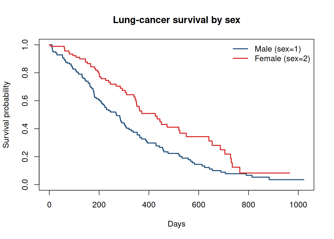
The exp(coef) column is the hazard ratio — $> 1$ increases hazard (shorter survival), $< 1$ decreases it. Here sex = 2 (female) has hazard ratio less than 1 — women in this dataset survived longer.

Kaplan-Meier — censored-data visualization

km_fit <- survfit(Surv(time, status) ~ sex, data = lung)

plot(km_fit, col = c("#1f4e79", "#d62828"), lwd = 2,
     xlab = "Days", ylab = "Survival probability",
     main = "Lung-cancer survival by sex")
legend("topright",
       legend = c("Male (sex=1)", "Female (sex=2)"),
       col = c("#1f4e79", "#d62828"), lwd = 2, bty = "n")

Figure 1: Kaplan-Meier survival curves by sex. The vertical ticks are *censored* observations — patients still alive when the study ended.

Tip

Censored data — the defining feature of survival analysis. A patient still alive when the study ends has “right-censored” survival time. Cox PH and Kaplan-Meier both handle this naturally; naive regression on survival time does not.

8. Gradient Boosting — Iterative Error Correction

Gradient boosting builds a strong learner by adding weak learners that each fit the residual errors of the current ensemble.

Pseudocode: 1. Start with $F_0(x)$ = a simple baseline (the mean works fine). 2. Compute the negative gradient of the loss at each training point. For squared error, this is just the residuals. 3. Fit a small learner $h_k(x)$ to those residuals. 4. Update: $F_{k+1}(x) = F_k(x) + \gamma \cdot h_k(x)$. 5. Repeat.

Let’s use the gbm package on a nonlinear regression problem.

suppressMessages(library(gbm))

set.seed(1)

n <- 500
x1 <- runif(n, -3, 3)
x2 <- runif(n, -3, 3)
y  <- sin(x1) + 0.5 * x2^2 + rnorm(n, 0, 0.3)

train_idx <- 1:400
train <- data.frame(x1, x2, y)[train_idx, ]
test  <- data.frame(x1, x2, y)[-train_idx, ]

fit_gbm <- gbm(y ~ x1 + x2, data = train,
               distribution = "gaussian",
               n.trees = 500, interaction.depth = 3,
               shrinkage = 0.05, verbose = FALSE)

pred <- predict(fit_gbm, newdata = test, n.trees = 500)
rmse <- sqrt(mean((test$y - pred)^2))
cat("Test RMSE:", round(rmse, 3), "\n")

Test RMSE: 0.355

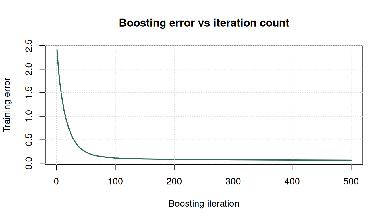
Figure 2: Training error as a function of number of boosting iterations. Classic shape: error drops fast, then plateaus. Stop too early and you underfit; go too long and you overfit.

A Tiny Hand-Worked Gradient Boosting Example

This toy example walks through four data points and shows one full boosting iteration converging from squared error 2.0 to 0.04 with an optimal step size $\gamma^* = 0.56$. Let’s replicate the key move — optimizing $\gamma$ analytically — on a toy dataset.

# Four points: F_0 predictions and residuals
y_true   <- c( 4,  5,  3,  1)
F_0_pred <- c(3.5, 5.5, 2.0, 1.5)   # base model predictions
residuals <- y_true - F_0_pred
residuals

[1]  0.5 -0.5  1.0 -0.5

# Imagine H_0 perfectly fits the residuals (it usually won't)
H_0_pred <- residuals

# Find optimal step size gamma for F_1 = F_0 + gamma * H_0
# Loss = sum((y - (F_0 + gamma * H_0))^2)
# dLoss/dgamma = -2 * sum(H_0 * (y - F_0 - gamma * H_0)) = 0
# => gamma = sum(H_0 * (y - F_0)) / sum(H_0^2)
gamma_star <- sum(H_0_pred * (y_true - F_0_pred)) / sum(H_0_pred^2)
cat("Optimal gamma:", round(gamma_star, 4), "\n")

Optimal gamma: 1

F_1_pred <- F_0_pred + gamma_star * H_0_pred
sse_before <- sum((y_true - F_0_pred)^2)
sse_after  <- sum((y_true - F_1_pred)^2)

cat("SSE before boosting step:", round(sse_before, 4), "\n")

SSE before boosting step: 1.75

cat("SSE after  boosting step:", round(sse_after,  4), "\n")

SSE after  boosting step: 0

When $H_0$ perfectly fits the residuals, $\gamma^* = 1$ and the error drops to zero. With imperfect fit (realistic case), $\gamma^*$ is smaller and the error drops by less — but every iteration improves the prediction.

Cheat Sheet

Topic	When to use	Key R tool
McNemar	Two paired binary outcomes	`mcnemar.test()`
Wilcoxon	Medians (paired or one-sample)	`wilcox.test(paired = TRUE)`
Mann-Whitney	Two independent distributions	`wilcox.test()`
Empirical Bayes	Lots of general data + little specific data	compute shrinkage by hand
Louvain	Find communities in a graph	`igraph::cluster_louvain()` (not shown — install for real use)
Neural network	Pattern recognition where rules aren’t expressible	`nnet::nnet()`
Game theory	Agents who react to your decisions	enumerate payoff matrix
NLP	Unstructured language data	`tm` / `quanteda` / transformers
Cox PH	Time-to-event with covariates	`survival::coxph()`
Gradient boosting	Tabular prediction with complex interactions	`gbm` / `xgboost`

Warning

Common pitfalls recap:

Base rate fallacy. Even a 98% sensitive test on a 1% prevalence disease gives only ~11% posterior probability of disease after a positive result.
Shrinkage is not intuitive. Extreme observed margins usually mean noise, not talent gaps.
Paired vs unpaired. Wilcoxon has both forms — pick based on whether the data comes in matched pairs.
Censoring. Never run plain regression on survival data — it discards the information from still-alive subjects.
Boosting overfits. Training error monotonically decreases but test error eventually climbs. Use early stopping or CV to pick number of iterations.
Game-theoretic equilibria are not always cooperative. The prisoner’s dilemma equilibrium is worse for everyone than the cooperative outcome.