Optimization: Variables, Constraints, and the Art of Modeling
Linear programming, binary variables, and why the modeling matters more than the solver
The Prescriptive Turn
Most of this guide so far has answered what will happen? Optimization answers what should we do? Given a goal, some constraints, and a set of decisions we control, what combination of decisions is best?
Two uses of optimization to remember:
Top-level prescriptive analytics — what should we invest in, how should we schedule workers, which route should the delivery truck take?
Underneath almost every model in this guide — linear regression, LASSO, ridge, logistic regression, SVM, exponential smoothing, ARIMA, GARCH, k-means — all are optimization problems being solved to pick parameters.
Tip
The big insight: software can solve optimization problems, but software cannot formulate them for you. The modeling is the hard part — and that makes it a competitive skill.
The Three Pieces of Every Optimization Model
Piece
What it represents
Variables
The decisions the solver picks values for
Constraints
The rules those decisions must obey
Objective function
The single number we’re maximizing or minimizing
A solution = a value for every variable. A feasible solution satisfies every constraint. The optimal solution is the feasible solution with the best objective value.
Warning
A useful language habit: never say “more optimal” or “most optimal.” It’s like saying “more best.” A solution is either optimal or it isn’t.
A Tiny LP: The Diet Problem
The original problem that kicked off linear programming in the 1940s: feed soldiers at minimum cost subject to nutritional constraints. Here’s a two-food, two-nutrient version.
Decision: how much of each food to serve. - \(x_1\) = servings of bread - \(x_2\) = servings of cheese
Constraints: need at least 8 g of protein and 10 g of carbs per meal. - Bread: 2 g protein, 4 g carbs per serving - Cheese: 5 g protein, 1 g carbs per serving
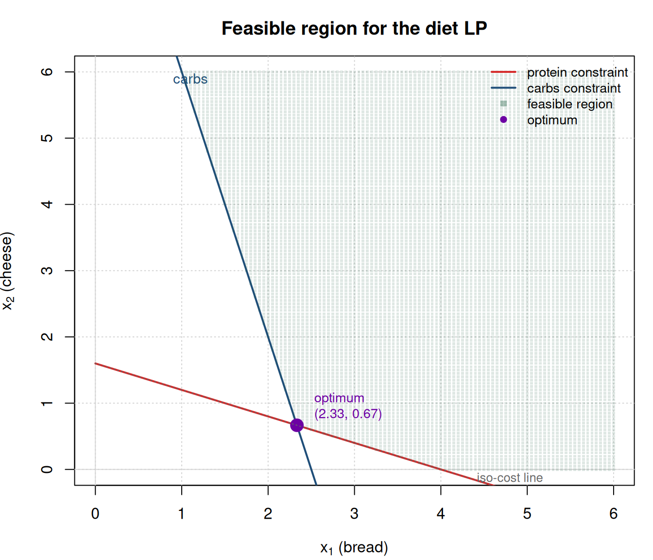
The Feasible Region — Seeing Why the Optimum Is at a Corner
For two-variable LPs, we can draw the feasible region.
Figure 1: Feasible region for the diet LP. Each constraint cuts off a half-plane; the feasible set is their intersection. The optimum of a linear objective lives at a vertex of this region.
Note
Check your understanding: Why does the optimum of an LP always sit at a vertex of the feasible region?
Answer: because the objective is linear. Moving along any edge changes the objective monotonically — you can always improve by going to a vertex. That’s the entire idea behind the simplex algorithm, which walks from vertex to vertex until no neighbor improves the objective.
The Variable-Choice Trap: Call Center Scheduling
Picking the right variables matters more than the algebra. The canonical scheduling warning is a call center that needs \(d_i\) workers on day \(i\) of the week and wants everyone to work 5 consecutive days before 2 off.
“Obvious” variables — \(x_i\) = number of workers on day \(i\): - Objective (\(\sum x_i\)) and demand (\(x_i \ge d_i\)) are trivial to write. - The 5-consecutive-days rule is nearly impossible to express.
Correct variables — \(x_i\) = number of workers who start their 5-day stretch on day \(i\): - Objective becomes \(5 \sum x_i\). - Tuesday demand is \(x_{\text{Fri}} + x_{\text{Sat}} + x_{\text{Sun}} + x_{\text{Mon}} + x_{\text{Tue}} \ge d_{\text{Tue}}\). - The 5-in-a-row rule is built into the variable definition — zero extra constraints needed.
Let’s solve it.
days <-c("Mon", "Tue", "Wed", "Thu", "Fri", "Sat", "Sun")# Demand forecastdemand <-c(Mon =17, Tue =13, Wed =15, Thu =19, Fri =14, Sat =16, Sun =11)# Variables: x[i] = workers starting their 5-day stretch on day i# Each x[i] covers 5 consecutive days starting at i (wrapping around the week)# Build the coverage matrix: rows = days of demand, cols = start daysn_days <-7coverage <-matrix(0, nrow = n_days, ncol = n_days)for (start in1:n_days) { covered <- ((start -1) +0:4) %% n_days +1 coverage[covered, start] <-1}dimnames(coverage) <-list(day_of_demand = days, start_day = days)coverage
Common pitfall: optimization is as much about problem formulation as about solving. The same problem, written with the wrong variables, can become intractable. Whenever a constraint feels awkward to write, consider whether a different variable definition would make it disappear.
Binary Variables: Fixed Charges and Logical Rules
Introducing \(y_i \in \{0, 1\}\) (1 if we invest in stock \(i\), 0 otherwise) lets us model real constraints that are impossible with continuous variables alone.
Fixed charges (transaction fees)
If buying any amount of a stock costs a flat transaction fee \(t\), add \(\sum_i t \cdot y_i\) to the objective, and link: \(x_i \le B \cdot y_i\) (if not buying, must be zero; if buying, up to budget \(B\)).
Minimum investment size
\(x_i \ge m_i \cdot y_i\) — can’t put $3 into Google because one share is hundreds.
Logical rules
Rule
Constraint
Must invest in Tesla
\(y_{\text{TSLA}} = 1\)
Invest in at least one of {A, G, AP}
\(y_A + y_G + y_{AP} \ge 1\)
Exactly one of them
\(y_A + y_G + y_{AP} = 1\)
FedEx and UPS together or neither
\(y_{\text{FDX}} = y_{\text{UPS}}\)
Coke and Pepsi opposite decisions
\(y_{\text{KO}} = 1 - y_{\text{PEP}}\)
Let’s solve a small portfolio problem that uses some of these.
stocks <-c("TSLA", "AMZN", "GOOG", "AAPL", "FDX", "UPS")returns <-c(0.18, 0.15, 0.12, 0.14, 0.09, 0.08) # expected return (decimal)budget <-100000min_invest <-5000# can't invest less than $5k per stocktxn_fee <-150# fixed fee per stock we pick# Decision variables: x1..x6 (dollars in each) then y1..y6 (binary pick)# Maximize: sum(returns * x) - sum(txn_fee * y)# Equivalently: minimize -(sum(returns * x) - sum(txn_fee * y))n <-length(stocks)objective <-c(-returns, rep(txn_fee, n)) # minimize# Constraints:# 1. Budget: sum(x_i) <= budget# 2. Linking (upper): x_i - budget * y_i <= 0 for each i# 3. Linking (lower min): x_i - min_invest * y_i >= 0 for each i# 4. At least one of {AMZN, GOOG, AAPL}: y_AMZN + y_GOOG + y_AAPL >= 1# 5. FedEx/UPS both or neither: y_FDX - y_UPS = 0# Budget rowA <-rbind(c(rep(1, n), rep(0, n)))dir <-c("<=")rhs <-c(budget)# Linking constraintsfor (i in1:n) { row_upper <-rep(0, 2* n) row_upper[i] <-1 row_upper[n + i] <--budget A <-rbind(A, row_upper); dir <-c(dir, "<="); rhs <-c(rhs, 0) row_lower <-rep(0, 2* n) row_lower[i] <-1 row_lower[n + i] <--min_invest A <-rbind(A, row_lower); dir <-c(dir, ">="); rhs <-c(rhs, 0)}# At least one of AMZN (2), GOOG (3), AAPL (4)one_of <-rep(0, 2* n)one_of[n +2] <-1; one_of[n +3] <-1; one_of[n +4] <-1A <-rbind(A, one_of); dir <-c(dir, ">="); rhs <-c(rhs, 1)# FDX (5) == UPS (6)both_or_neither <-rep(0, 2* n)both_or_neither[n +5] <-1both_or_neither[n +6] <--1A <-rbind(A, both_or_neither); dir <-c(dir, "="); rhs <-c(rhs, 0)sol_port <-lp(direction ="min",objective.in = objective,const.mat = A,const.dir = dir,const.rhs = rhs,int.vec = (n +1):(2* n), # y_i are integerbinary.vec = (n +1):(2* n) # and binary)x_vals <- sol_port$solution[1:n]y_vals <- sol_port$solution[(n +1):(2* n)]portfolio <-data.frame(stock = stocks,picked =as.logical(y_vals),invested =round(x_vals, 0),expected_return =round(x_vals * returns, 0))portfolio
cat("Expected return net of fees: $",round(sum(x_vals * returns) -sum(y_vals * txn_fee), 0), "\n")
Expected return net of fees: $ 17550
The solver picks the best set, respects the minimum-investment rule, includes at least one of {AMZN, GOOG, AAPL}, and treats FedEx/UPS as a matched pair.
The Problem-Type Hierarchy (Easiest → Hardest)
Type
Notes
Linear Program (LP)
Millions of variables, fast. What we’ve been doing.
Convex Quadratic Program (QP)
Fast. Portfolio optimization, ridge regression.
Convex Optimization (general)
Still “easy” in theory, can be slow.
Integer Program (IP)
Hard. Some small IPs don’t have known optimal solutions even after days of compute.
General Non-Convex
Brutal. Even tiny problems may be intractable.
Network Optimization
Faster than LP. Shortest path, assignment, max flow.
Tip
Recognizing the type matters. A problem written as an IP may be intractable, but the same problem re-formulated as a network-flow problem can solve in milliseconds. This is why modeling ability matters more than knowing how to call a solver.
Handling Uncertainty — Four Approaches
When input data is uncertain (demand forecasts, returns, transition rates), the deterministic optimum can be catastrophically bad. Four approaches:
Approach
Idea
Conservative constraints
Pad the RHS: require demand + \(\theta\) extra buffer.
Chance constraints
\(P(\text{demand met}) \ge p\). Needs a distribution estimate.
Scenario optimization
Define multiple scenarios, solve for a robust solution (feasible in all) or minimize expected cost across them.
Model the system as states + decisions + transition probabilities and find the best policy via Bellman’s equation.
Scenario optimization in particular is very flexible — you can represent a messy probabilistic world as a discrete set of “what-ifs” and let the solver pick a policy that works across them.
Regression as Optimization — The Terminology Collision
Every regression, LASSO, ridge, logistic regression, SVM, exponential-smoothing, ARIMA, GARCH, and k-means model discussed in this guide is really an optimization problem inside. The confusing bit is terminology: statisticians call the data \(x_{ij}\) “variables” (they vary across rows); optimizers call the coefficients \(a_0, a_1, \ldots\) “variables” (they’re what the solver picks).
Let’s solve linear regression explicitly as optimization to drive the point home.
Same answer. The optim() version is doing what lm() does under the hood — it just exposes the optimization nature. And because it’s an optimization problem, we can customize it: force the intercept to zero, constrain coefficients to be monotone, use \(|y - \hat{y}|^{1.5}\) instead of squared error, etc. Standard regression packages can’t do that; optimization solvers can.
Cheat Sheet
Warning
Common pitfalls recap:
“More optimal” is not a thing. A solution is optimal or it isn’t.
Problem formulation > solver choice. The call-center example is the canonical illustration.
Link the variables. Solvers only see math, not your English intent. \(\sum_d v_{id} = y_i\) may be invisible to the solver if you don’t write it.
LP optima live at vertices. That’s why simplex works.
Binary variables make IPs hard. Don’t default to “\(y \in \{0, 1\}\)” without considering whether an LP or network formulation would do.
Regression is optimization in disguise. So are LASSO, SVM, exponential smoothing, and k-means. Knowing this lets you customize them.
Statisticians and optimizers mean different things by “variable.” Always check which hat the person is wearing.