CUSUM From Scratch: Catching the Moment Everything Changed

Change detection — when did the process shift?

1. The Problem: Did Something Change?

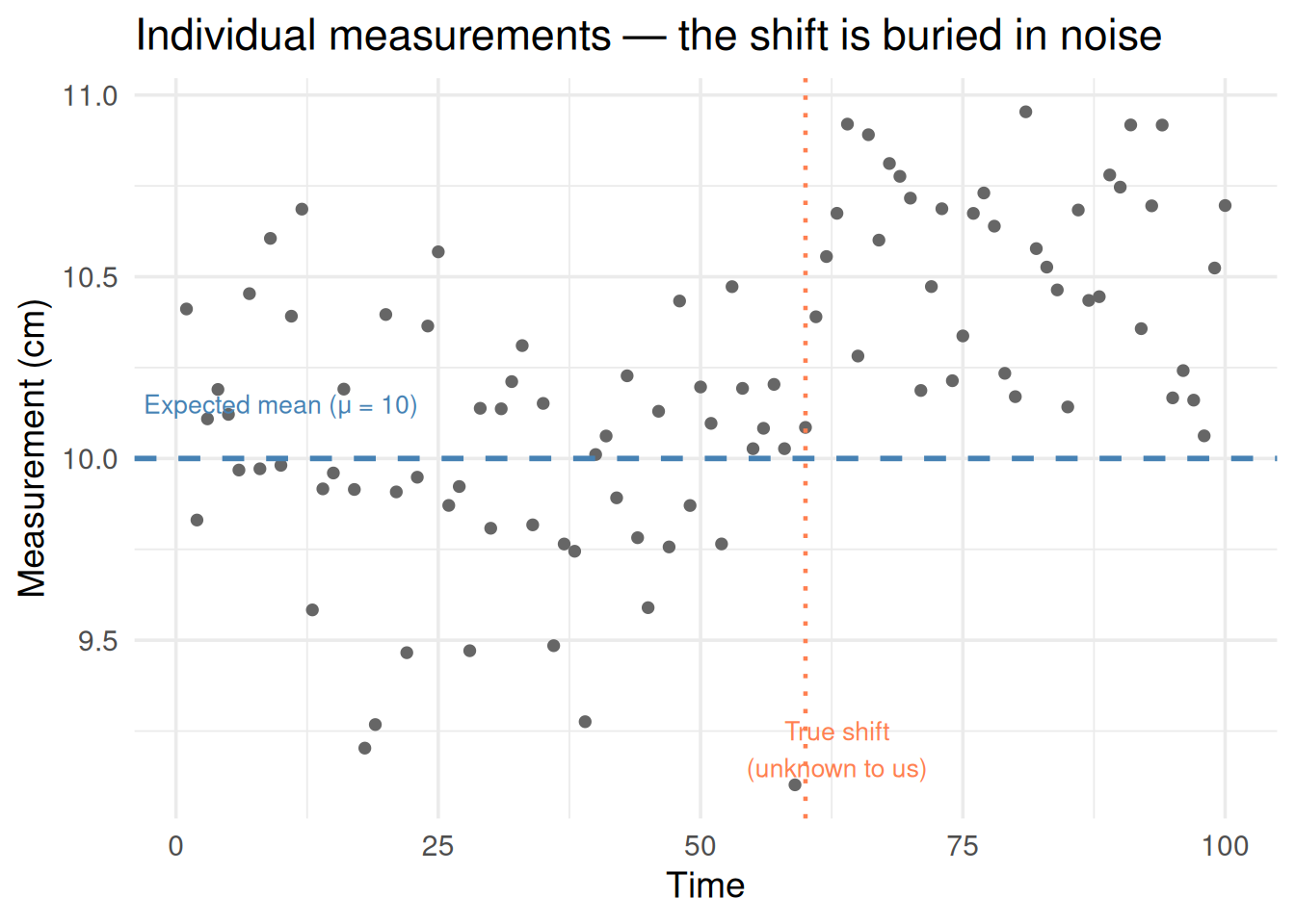
A factory makes bolts that should be exactly 10 cm long. Every hour you measure a bolt. The measurements bounce around a little — that’s normal random variation. But at some point, the machine drifts and starts making bolts that are slightly too long.

When did the change happen?

You can’t just look at one measurement — any single value might be high by chance. You need a method that accumulates evidence over time and shouts “something changed!” only when it’s confident.

That’s CUSUM.

library(ggplot2)
set.seed(42)

# Normal process, then a shift at t = 60
n <- 100
mu <- 10       # expected mean
shift <- 0.5   # how much the mean shifts

x <- c(rnorm(60, mu, 0.3), rnorm(40, mu + shift, 0.3))
time <- 1:n

df <- data.frame(time = time, value = x)

ggplot(df, aes(time, value)) +
  geom_point(color = "gray40", size = 1.5) +
  geom_hline(yintercept = mu, color = "steelblue", linewidth = 1, linetype = "dashed") +
  annotate("text", x = 10, y = mu + 0.15, label = "Expected mean (μ = 10)",
           color = "steelblue", size = 3.5) +
  geom_vline(xintercept = 60, color = "coral", linetype = "dotted", linewidth = 0.8) +
  annotate("text", x = 63, y = 9.2, label = "True shift\n(unknown to us)",
           color = "coral", size = 3.5) +
  theme_minimal(base_size = 14) +
  labs(x = "Time", y = "Measurement (cm)",
       title = "Individual measurements — the shift is buried in noise")

Figure 1: Can you spot where the process shifted? It’s hard to tell from individual points.

Each point looks reasonable on its own. The shift is only 0.5 cm in a process with 0.3 cm of natural variation. CUSUM will find it.

2. The Idea: Keep a Running Score

CUSUM stands for CUmulative SUM. The idea:

1. Start with a score of zero
2. Each time step, check: is this observation above what we expect?
3. If yes, add to the score (evidence is accumulating)
4. If no, subtract from the score (but never go below zero)
5. When the score crosses a threshold → declare a change

It’s like a detective building a case. Each above-average observation is a small piece of evidence. One piece isn’t convincing. But when evidence keeps piling up, eventually you’re confident something changed.

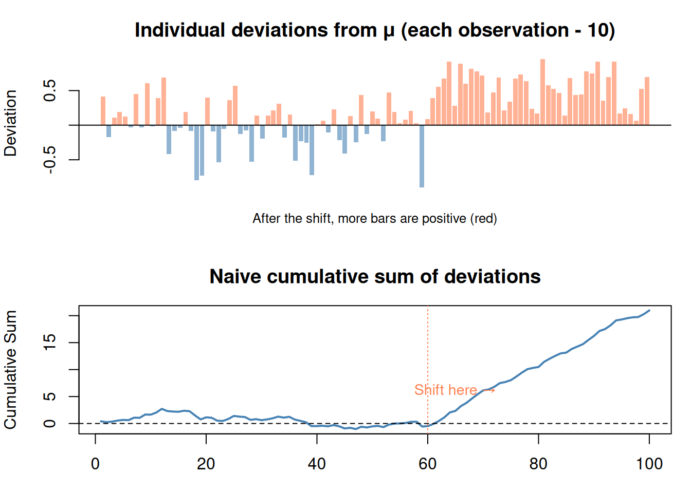
# Simple visual: show deviations accumulating
deviations <- x - mu

colors <- ifelse(deviations > 0, "coral", "steelblue")

par(mfrow = c(2, 1), mar = c(3, 4, 3, 1))

# Top: individual deviations
barplot(deviations, col = adjustcolor(colors, 0.6), border = NA,
  main = "Individual deviations from μ (each observation - 10)",
  ylab = "Deviation", names.arg = rep("", n))
abline(h = 0)
mtext("After the shift, more bars are positive (red)", side = 1, line = 1, cex = 0.8)

# Bottom: cumulative sum
cumdev <- cumsum(deviations)
plot(time, cumdev, type = "l", lwd = 2, col = "steelblue",
  main = "Naive cumulative sum of deviations",
  ylab = "Cumulative Sum", xlab = "Time")
abline(h = 0, lty = 2)
abline(v = 60, col = "coral", lty = 3)
text(65, max(cumdev) * 0.3, "Shift here →", col = "coral", cex = 0.9)

par(mfrow = c(1, 1))

Figure 2: CUSUM accumulates positive deviations. When they pile up, a change is detected.

The naive cumulative sum shows the trend, but it’s noisy before the shift because random below-average values create a downward drift. CUSUM fixes this with two clever additions: the allowance (C) and the floor at zero.

3. The CUSUM Formula

\[S_t = \max(0, \; S_{t-1} + (x_t - \mu) - C)\]

Declare a change when \(S_t > T\)

That’s the whole formula. Let’s unpack every piece:

Symbol	What it is	Plain English
\(S_t\)	CUSUM statistic at time \(t\)	The running score (accumulated evidence)
\(S_{t-1}\)	Previous score	What we had so far
\(x_t\)	Current observation	The new measurement
\(\mu\)	Expected mean	What the process should be producing
\(x_t - \mu\)	Deviation	How far this observation is from expected
\(C\)	Allowance (critical value)	Filters out normal noise — only counts “big enough” deviations
\(\max(0, \dots)\)	Floor at zero	Prevents negative accumulation — past good behavior doesn’t mask future problems
\(T\)	Threshold	How much evidence you need before declaring a change

Step by Step

At each time step:

1. Take the new observation \(x_t\)
2. Compute the deviation: \(x_t - \mu\) (how far from expected?)
3. Subtract the allowance \(C\) (ignore small, normal fluctuations)
4. Add to previous score \(S_{t-1}\)
5. If the result is negative, reset to 0 (fresh start)
6. If \(S_t > T\), sound the alarm

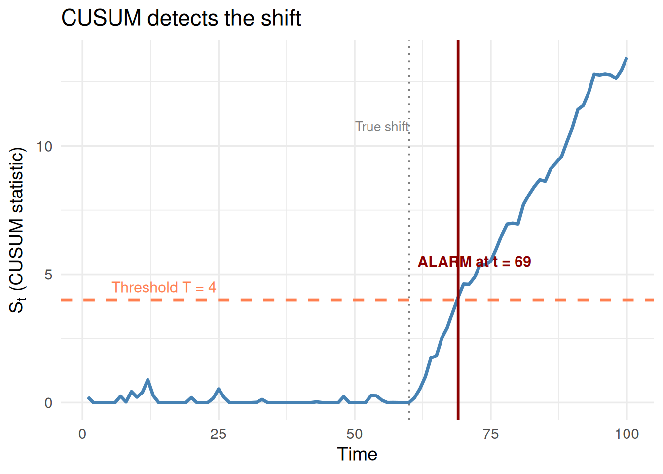
# Compute CUSUM
C_val <- 0.2  # allowance
T_val <- 4    # threshold

S <- numeric(n)
S[1] <- max(0, (x[1] - mu) - C_val)

for (t in 2:n) {
  S[t] <- max(0, S[t - 1] + (x[t] - mu) - C_val)
}

# When does it cross T?
alarm_time <- which(S > T_val)[1]

df_cusum <- data.frame(time = time, S = S)

ggplot(df_cusum, aes(time, S)) +
  geom_line(linewidth = 1.2, color = "steelblue") +
  geom_hline(yintercept = T_val, color = "coral", linewidth = 1, linetype = "dashed") +
  annotate("text", x = 15, y = T_val + 0.5,
           label = paste0("Threshold T = ", T_val), color = "coral", size = 4) +
  geom_vline(xintercept = 60, color = "gray50", linetype = "dotted") +
  annotate("text", x = 55, y = max(S) * 0.8, label = "True shift", color = "gray50", size = 3.5) +
  { if (!is.na(alarm_time))
    list(
      geom_vline(xintercept = alarm_time, color = "darkred", linewidth = 1),
      annotate("text", x = alarm_time + 3, y = T_val + 1.5,
               label = paste0("ALARM at t = ", alarm_time),
               color = "darkred", fontface = "bold", size = 4)
    )
  } +
  theme_minimal(base_size = 14) +
  labs(x = "Time", y = expression(S[t] ~ "(CUSUM statistic)"),
       title = "CUSUM detects the shift")

Figure 3: CUSUM in action: the score accumulates after the shift and crosses the threshold

4. What C and T Do (The Two Knobs)

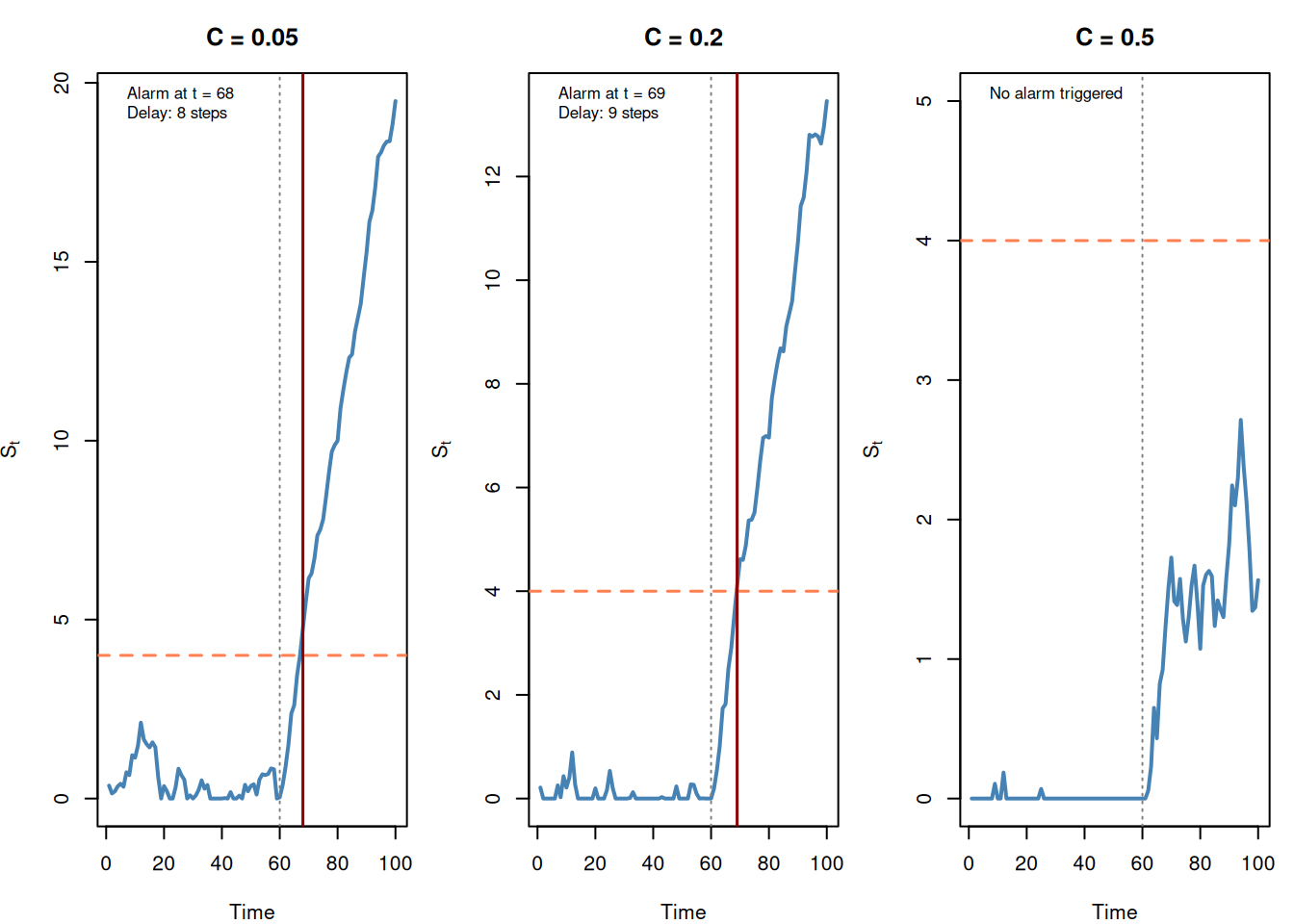
C (Allowance): How Much Noise to Ignore

\(C\) is a filter. It subtracts from each deviation so that normal random fluctuations don’t accumulate.

• Large C: Only big deviations count → slower detection, fewer false alarms
• Small C: Small deviations count → faster detection, more false alarms
• C = 0: Every above-average observation adds to the score (very sensitive)

par(mfrow = c(1, 3), mar = c(4, 4, 3, 1))

for (C_test in c(0.05, 0.2, 0.5)) {
  S_test <- numeric(n)
  S_test[1] <- max(0, (x[1] - mu) - C_test)
  for (t in 2:n) {
    S_test[t] <- max(0, S_test[t - 1] + (x[t] - mu) - C_test)
  }

  alarm <- which(S_test > T_val)[1]

  plot(time, S_test, type = "l", lwd = 2, col = "steelblue",
    main = paste0("C = ", C_test),
    xlab = "Time", ylab = expression(S[t]),
    ylim = c(0, max(S_test, T_val + 1)))
  abline(h = T_val, col = "coral", lty = 2, lwd = 1.5)
  abline(v = 60, col = "gray50", lty = 3)

  if (!is.na(alarm)) {
    abline(v = alarm, col = "darkred", lwd = 1.5)
    legend("topleft", bty = "n", cex = 0.8,
      legend = c(
        paste0("Alarm at t = ", alarm),
        paste0("Delay: ", alarm - 60, " steps")
      ))
  } else {
    legend("topleft", bty = "n", cex = 0.8, legend = "No alarm triggered")
  }
}
par(mfrow = c(1, 1))

Figure 4: Larger C = slower detection but fewer false alarms

T (Threshold): How Much Evidence Before Alarm

\(T\) controls how certain you need to be before declaring a change.

• Large T: Need lots of evidence → fewer false alarms, but slower detection
• Small T: Trigger on less evidence → faster detection, more false alarms

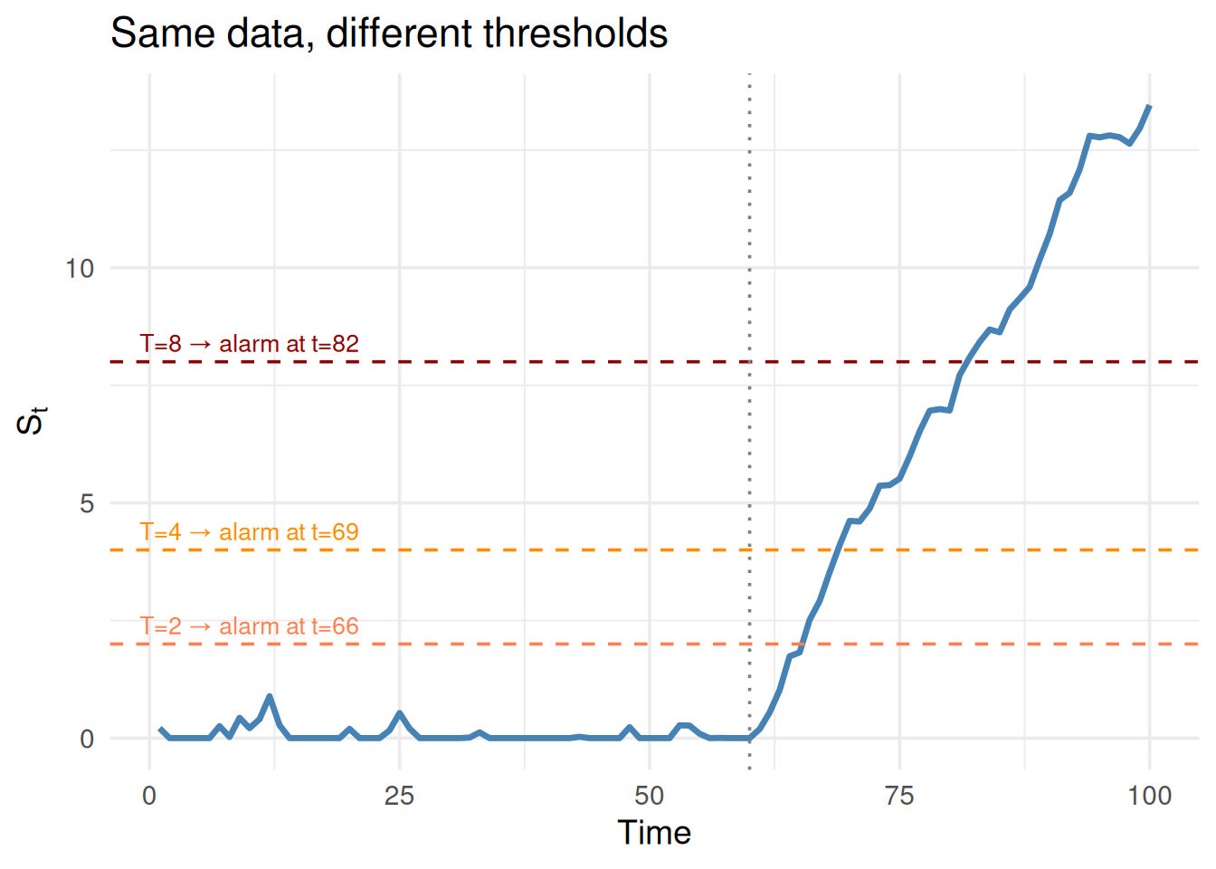
# Fix C, vary T
C_fixed <- 0.2

S_fixed <- numeric(n)
S_fixed[1] <- max(0, (x[1] - mu) - C_fixed)
for (t in 2:n) {
  S_fixed[t] <- max(0, S_fixed[t - 1] + (x[t] - mu) - C_fixed)
}

T_vals <- c(2, 4, 8)
alarm_times <- sapply(T_vals, function(Tv) which(S_fixed > Tv)[1])

df_t <- data.frame(time = time, S = S_fixed)

ggplot(df_t, aes(time, S)) +
  geom_line(linewidth = 1.2, color = "steelblue") +
  geom_hline(yintercept = T_vals[1], color = "coral", linetype = "dashed") +
  geom_hline(yintercept = T_vals[2], color = "darkorange", linetype = "dashed") +
  geom_hline(yintercept = T_vals[3], color = "darkred", linetype = "dashed") +
  annotate("text", x = 10, y = T_vals[1] + 0.4,
           label = paste0("T=2 → alarm at t=", alarm_times[1]), color = "coral", size = 3.5) +
  annotate("text", x = 10, y = T_vals[2] + 0.4,
           label = paste0("T=4 → alarm at t=", alarm_times[2]), color = "darkorange", size = 3.5) +
  annotate("text", x = 10, y = T_vals[3] + 0.4,
           label = paste0("T=8 → alarm at t=",
                          ifelse(is.na(alarm_times[3]), "never", alarm_times[3])),
           color = "darkred", size = 3.5) +
  geom_vline(xintercept = 60, color = "gray50", linetype = "dotted") +
  theme_minimal(base_size = 14) +
  labs(x = "Time", y = expression(S[t]),
       title = "Same data, different thresholds")

Figure 5: Larger T = more evidence needed before triggering an alarm

5. The Speed vs. False Alarm Tradeoff

This is the central tradeoff to understand. There’s no free lunch.

     Fast detection                    Slow detection
     More false alarms                 Fewer false alarms
     ◄─────────────────────────────────────────────────►
     Small C, Small T                  Large C, Large T

The right C and T depend on the costs:

Scenario	Want	Set
Nuclear reactor monitoring	Fast detection (safety!)	Small C, small T
Marketing campaign tracking	Few false alarms (budget!)	Large C, large T
Manufacturing quality	Balance both	Moderate C and T

WarningCommon Pitfall: T and C Parameters

“What happens if we increase T?” → Fewer false alarms, slower detection. “What happens if we increase C?” → Same effect. There’s no universal best value — it depends on the application.

6. Why max(0, …) Matters

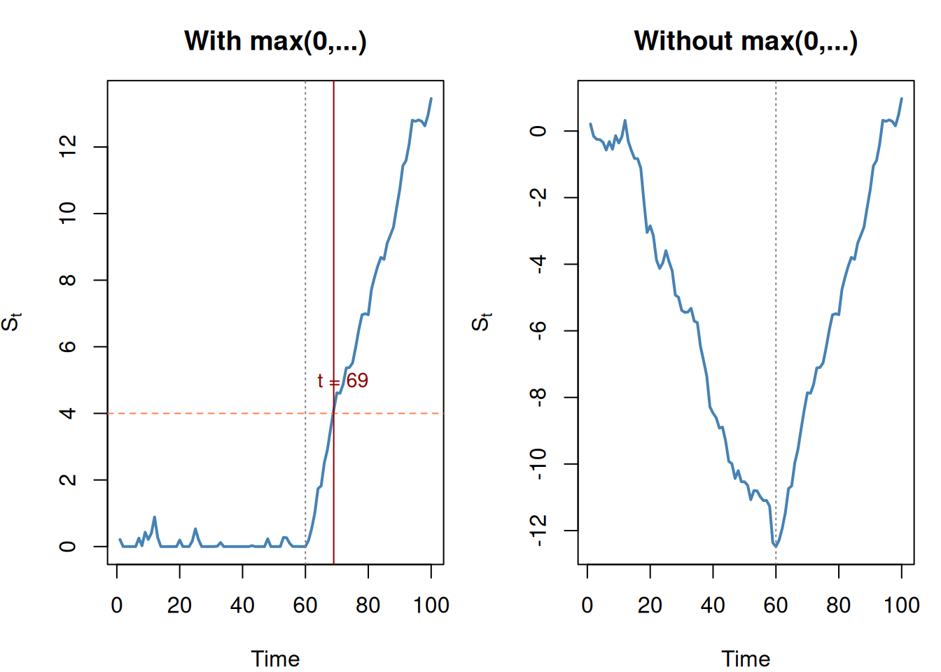
The floor at zero is crucial. Without it, a long stretch of below-average values would build up a large negative score. Then when a real shift happens, the score has to climb back from that hole before triggering an alarm.

C_demo <- 0.2

# With max(0, ...)
S_with <- numeric(n)
S_with[1] <- max(0, (x[1] - mu) - C_demo)
for (t in 2:n) {
  S_with[t] <- max(0, S_with[t - 1] + (x[t] - mu) - C_demo)
}

# Without max(0, ...) — naive version
S_without <- numeric(n)
S_without[1] <- (x[1] - mu) - C_demo
for (t in 2:n) {
  S_without[t] <- S_without[t - 1] + (x[t] - mu) - C_demo
}

par(mfrow = c(1, 2), mar = c(4, 4, 3, 1))

plot(time, S_with, type = "l", lwd = 2, col = "steelblue",
  main = "With max(0,...)",
  xlab = "Time", ylab = expression(S[t]))
abline(h = T_val, col = "coral", lty = 2)
abline(v = 60, col = "gray50", lty = 3)
alarm1 <- which(S_with > T_val)[1]
if (!is.na(alarm1)) {
  abline(v = alarm1, col = "darkred")
  text(alarm1 + 3, T_val + 1, paste("t =", alarm1), col = "darkred", cex = 0.9)
}

plot(time, S_without, type = "l", lwd = 2, col = "steelblue",
  main = "Without max(0,...)",
  xlab = "Time", ylab = expression(S[t]))
abline(h = T_val, col = "coral", lty = 2)
abline(v = 60, col = "gray50", lty = 3)
alarm2 <- which(S_without > T_val)[1]
if (!is.na(alarm2)) {
  abline(v = alarm2, col = "darkred")
  text(alarm2 + 3, T_val + 1, paste("t =", alarm2), col = "darkred", cex = 0.9)
}

par(mfrow = c(1, 1))

Figure 6: Without max(0,…), past good behavior delays detection of real changes

The version without max(0,...) digs into a negative hole during the normal period, then takes longer to climb back up after the shift. The proper CUSUM resets to zero whenever it would go negative — every moment is a potential fresh start for detecting a change.

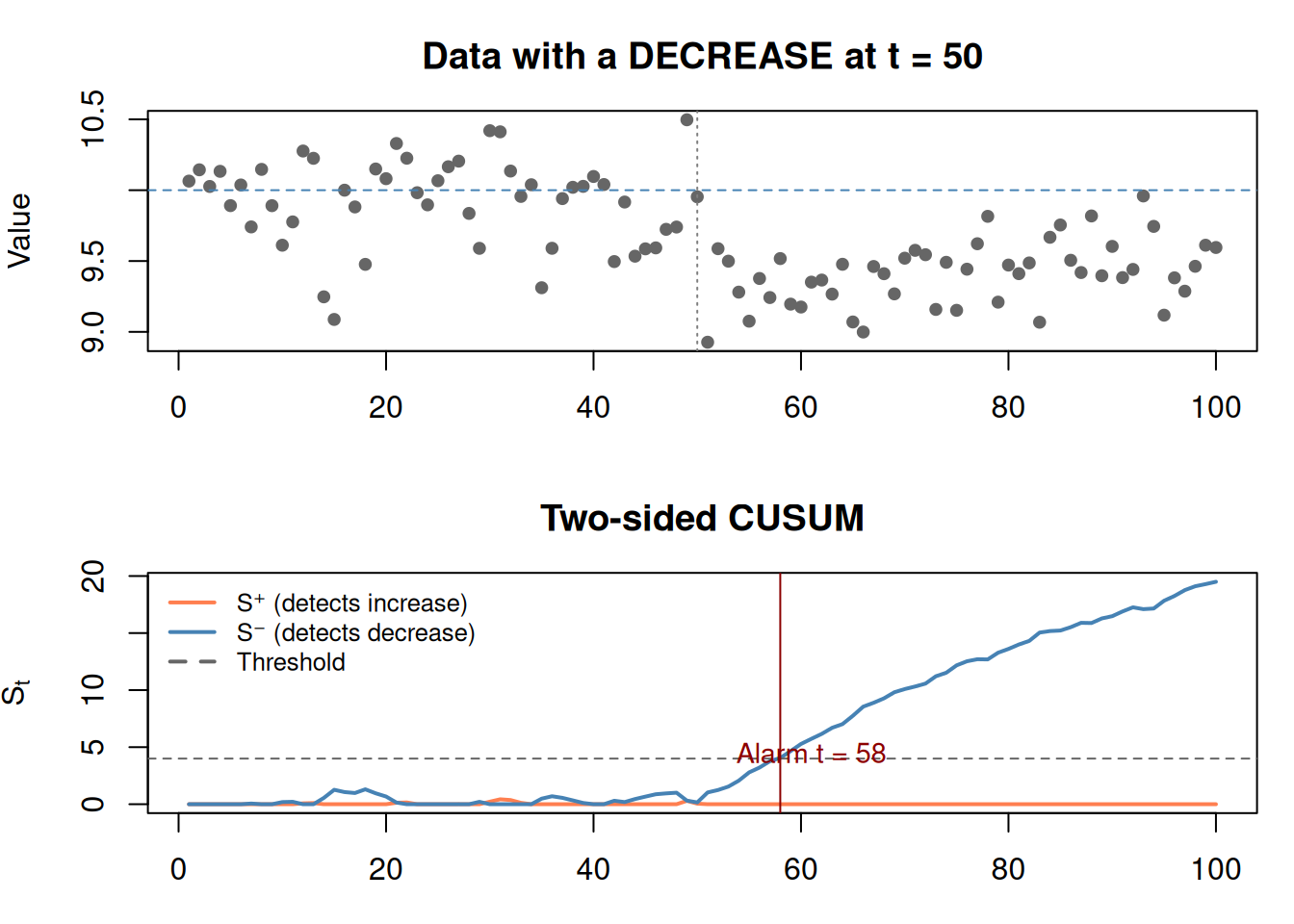
7. Detecting Decreases (Two-Sided CUSUM)

The formula above only detects increases (upward shifts). To detect decreases, run a second CUSUM in the other direction:

\[S_t^+ = \max(0, \; S_{t-1}^+ + (x_t - \mu) - C) \quad \text{(detects increase)}\] \[S_t^- = \max(0, \; S_{t-1}^- - (x_t - \mu) - C) \quad \text{(detects decrease)}\]

Alarm when either \(S_t^+ > T\) or \(S_t^- > T\).

set.seed(99)

# Process with a DECREASE at t=50
x2 <- c(rnorm(50, 10, 0.3), rnorm(50, 9.4, 0.3))

S_up <- numeric(n)
S_down <- numeric(n)
C2 <- 0.2

for (t in 2:n) {
  S_up[t] <- max(0, S_up[t - 1] + (x2[t] - mu) - C2)
  S_down[t] <- max(0, S_down[t - 1] - (x2[t] - mu) - C2)
}

par(mfrow = c(2, 1), mar = c(3, 4, 3, 1))

plot(time, x2, pch = 19, cex = 0.8, col = "gray40",
  main = "Data with a DECREASE at t = 50",
  ylab = "Value", xlab = "")
abline(h = mu, col = "steelblue", lty = 2)
abline(v = 50, col = "gray50", lty = 3)

plot(time, S_up, type = "l", lwd = 2, col = "coral",
  ylim = c(0, max(c(S_up, S_down, T_val + 1))),
  main = "Two-sided CUSUM", ylab = expression(S[t]), xlab = "Time")
lines(time, S_down, lwd = 2, col = "steelblue")
abline(h = T_val, lty = 2, col = "gray40")
legend("topleft", bty = "n",
  legend = c("S⁺ (detects increase)", "S⁻ (detects decrease)", "Threshold"),
  col = c("coral", "steelblue", "gray40"), lty = c(1, 1, 2), lwd = 2, cex = 0.8)

alarm_down <- which(S_down > T_val)[1]
if (!is.na(alarm_down)) {
  abline(v = alarm_down, col = "darkred")
  text(alarm_down + 3, T_val + 0.5, paste("Alarm t =", alarm_down),
       col = "darkred", cex = 0.9)
}

par(mfrow = c(1, 1))

Figure 7: Two-sided CUSUM catches both upward and downward shifts

8. CUSUM Cannot Tell You WHY

WarningCommon Pitfall: CUSUM Cannot Tell You WHY

CUSUM tells you when something changed. It does not tell you what changed or why.

“CUSUM detected a shift in manufacturing quality at day 60.”

Wrong conclusion: “The machine is broken.”

Right conclusion: “Something changed around day 60. We need to investigate what happened.”

CUSUM is a detection tool, not a diagnosis tool. The investigation happens after the alarm.

9. Real-World Applications

Application	What \(x_t\) measures	What “change” means
Manufacturing	Part dimension	Machine needs recalibration
Healthcare	Patient vitals	Condition is deteriorating
Finance	Transaction amounts	Potential fraud pattern
Website	Page load times	Server performance degraded
Retail	Daily sales	Market shift or competitor action

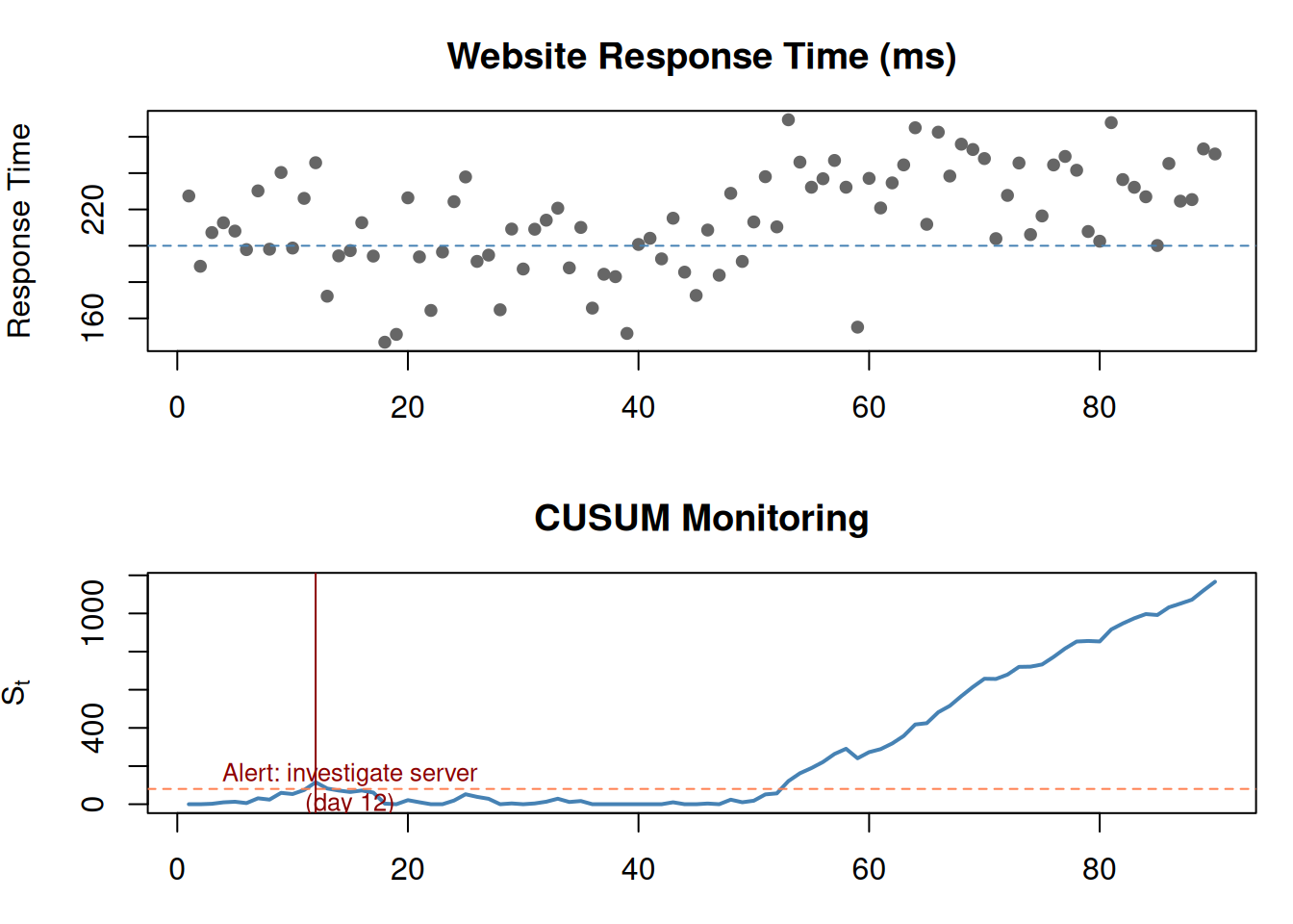
set.seed(42)

# Website response time (ms)
days <- 1:90
resp_time <- c(
  rnorm(50, 200, 20),   # normal
  rnorm(40, 230, 25)    # degraded after day 50
)

mu_web <- 200
C_web <- 5
T_web <- 80

S_web <- numeric(90)
for (t in 2:90) {
  S_web[t] <- max(0, S_web[t - 1] + (resp_time[t] - mu_web) - C_web)
}

alarm_web <- which(S_web > T_web)[1]

par(mfrow = c(2, 1), mar = c(3, 4, 3, 1))

plot(days, resp_time, pch = 19, cex = 0.8, col = "gray40",
  main = "Website Response Time (ms)",
  ylab = "Response Time", xlab = "")
abline(h = mu_web, col = "steelblue", lty = 2)

plot(days, S_web, type = "l", lwd = 2, col = "steelblue",
  main = "CUSUM Monitoring", ylab = expression(S[t]), xlab = "Day")
abline(h = T_web, col = "coral", lty = 2)
if (!is.na(alarm_web)) {
  abline(v = alarm_web, col = "darkred")
  text(alarm_web + 3, T_web + 10,
    paste0("Alert: investigate server\n(day ", alarm_web, ")"),
    col = "darkred", cex = 0.8)
}

par(mfrow = c(1, 1))

Figure 8: CUSUM applied to website response times — detects server degradation

10. CUSUM vs Other Methods

Method	Detects	When to use
CUSUM	Shift in process mean	Ongoing monitoring, small persistent shifts
Control chart	Individual outlier points	Quick spikes, obvious violations
t-test	Difference between two groups	Comparing before/after with known breakpoint
Exponential smoothing	Trends and patterns	Forecasting future values

CUSUM’s superpower is detecting small, gradual shifts that individual observations can’t catch. A single point might look normal, but CUSUM accumulates the evidence until the pattern is undeniable.

11. Cheat Sheet: The Whole Story on One Page

THE CUSUM RECIPE
=================

1. PURPOSE: Detect when a process mean has shifted

2. THE FORMULA:
   Sₜ = max(0, Sₜ₋₁ + (xₜ - μ) - C)

   Alarm when Sₜ > T

3. SYMBOLS:
   Sₜ  = accumulated evidence (running score)
   xₜ  = current observation
   μ   = expected baseline mean
   C   = allowance (noise filter)
   T   = threshold (alarm trigger)

4. KEY PARAMETERS:
   C → how much noise to ignore
   T → how much evidence needed for alarm
   Both: ↑ value = slower detection, fewer false alarms
         ↓ value = faster detection, more false alarms

5. WHY max(0,...)?
   Prevents past good behavior from masking future changes.
   Every moment is a fresh start for detection.

6. TWO-SIDED:
   S⁺ detects increases, S⁻ detects decreases

7. CUSUM CANNOT:
   - Tell you WHY something changed
   - Tell you WHAT changed
   - Only tells you WHEN

8. COMMON PITFALLS:
   - No universal best C and T (depends on costs)
   - "Increase T" → fewer false alarms, slower detection
   - CUSUM detects, it doesn't diagnose

12. Check Your Understanding

NoteTest Yourself

Before moving on, try to answer these without scrolling up:

1. What does CUSUM stand for and what does it detect?
2. Walk through the formula \(S_t = \max(0, S_{t-1} + (x_t - \mu) - C)\) in plain English.
3. What does \(C\) (allowance) control? What happens if you increase it?
4. What does \(T\) (threshold) control? What happens if you decrease it?
5. Why is the \(\max(0, \dots)\) necessary? What would happen without it?
6. CUSUM triggers an alarm. Can you conclude the machine is broken? Why or why not?
7. A nuclear power plant wants fast detection at all costs. A marketing team wants to avoid false alarms. How should each set C and T?
8. How is CUSUM different from just looking at individual measurements?