KNN From Scratch: Unpacking the Formula

The simplest idea in machine learning — and why it works

1. The Problem: Classify a New Point

You have labeled data — points that already belong to known groups. A new, unlabeled point shows up. Which group does it belong to?

library(ggplot2)
set.seed(42)

df <- data.frame(
  x1 = c(rnorm(30, 2, 0.7), rnorm(30, 5, 0.7)),
  x2 = c(rnorm(30, 2, 0.7), rnorm(30, 5, 0.7)),
  group = factor(rep(c("Red", "Blue"), each = 30))
)

new_point <- data.frame(x1 = 3.8, x2 = 3.5)

ggplot(df, aes(x1, x2, color = group)) +
  geom_point(size = 3) +
  geom_point(data = new_point, aes(x1, x2), color = "black",
             shape = 18, size = 6, inherit.aes = FALSE) +
  scale_color_manual(values = c("steelblue", "coral")) +
  annotate("text", x = 4.1, y = 3.2, label = "???", fontface = "bold", size = 5) +
  theme_minimal(base_size = 14) +
  labs(x = "Feature 1", y = "Feature 2")

Figure 1: A new point (black diamond) arrives. Which group does it belong to?

KNN’s answer is absurdly simple: look at the closest points and go with the majority vote.

That’s it. That’s the whole algorithm.

2. The Algorithm in Plain English

1. Pick a number \(k\) (e.g., 5)
2. Measure the distance from the new point to every training point
3. Find the \(k\) closest neighbors
4. Count how many belong to each class
5. The new point gets the class with the most votes

# Calculate distances from new point to all training points
df$dist <- sqrt((df$x1 - new_point$x1)^2 + (df$x2 - new_point$x2)^2)
df$rank <- rank(df$dist)
df$is_neighbor <- df$rank <= 5

# Count votes
neighbors <- df[df$is_neighbor, ]
vote_red <- sum(neighbors$group == "Red")
vote_blue <- sum(neighbors$group == "Blue")

ggplot(df, aes(x1, x2, color = group)) +
  geom_point(size = 3, alpha = 0.3) +
  # Highlight neighbors
  geom_point(data = neighbors, aes(x1, x2, color = group), size = 4) +
  # Draw lines from new point to neighbors
  geom_segment(data = neighbors,
    aes(x = new_point$x1, y = new_point$x2, xend = x1, yend = x2),
    color = "gray50", linetype = "dashed", inherit.aes = FALSE) +
  # New point
  geom_point(data = new_point, aes(x1, x2), color = "black",
             shape = 18, size = 6, inherit.aes = FALSE) +
  # Circle around neighborhood
  annotate("path",
    x = new_point$x1 + max(neighbors$dist) * cos(seq(0, 2*pi, length.out = 100)),
    y = new_point$x2 + max(neighbors$dist) * sin(seq(0, 2*pi, length.out = 100)),
    linetype = "dotted", color = "gray40") +
  scale_color_manual(values = c("steelblue", "coral")) +
  annotate("label", x = 5.5, y = 1.5, size = 4,
    label = paste0("Vote: ", vote_red, " Red, ", vote_blue, " Blue\n",
                   "Winner: ", ifelse(vote_red > vote_blue, "Red", "Blue"))) +
  theme_minimal(base_size = 14) +
  labs(x = "Feature 1", y = "Feature 2")

Figure 2: k=5: find 5 nearest neighbors, take majority vote

3. The Formula: Distance

The only math KNN needs is a way to measure how far apart two points are.

Euclidean Distance (the default)

\[d(\mathbf{x}, \mathbf{x}') = \sqrt{\sum_{j=1}^{p} (x_j - x_j')^2}\]

Symbol	What it is	Plain English
\(\mathbf{x}\)	The new point	The thing we’re classifying
\(\mathbf{x}'\)	A training point	One of the known, labeled examples
\(p\)	Number of features	How many measurements each point has
\(x_j\)	Feature \(j\) of the new point	e.g., income
\(x_j'\)	Feature \(j\) of the training point	e.g., that person’s income

In 2D, this is just the Pythagorean theorem:

\[d = \sqrt{(x_1 - x_1')^2 + (x_2 - x_2')^2}\]

p1 <- data.frame(x1 = 2, x2 = 1)
p2 <- data.frame(x1 = 5, x2 = 5)
d <- sqrt((p2$x1 - p1$x1)^2 + (p2$x2 - p1$x2)^2)

ggplot() +
  # The two points
  geom_point(data = p1, aes(x1, x2), size = 5, color = "coral") +
  geom_point(data = p2, aes(x1, x2), size = 5, color = "steelblue") +
  # Direct line (hypotenuse)
  geom_segment(aes(x = p1$x1, y = p1$x2, xend = p2$x1, yend = p2$x2),
               linewidth = 1.2) +
  # Horizontal leg
  geom_segment(aes(x = p1$x1, y = p1$x2, xend = p2$x1, yend = p1$x2),
               linetype = "dashed", color = "gray50") +
  # Vertical leg
  geom_segment(aes(x = p2$x1, y = p1$x2, xend = p2$x1, yend = p2$x2),
               linetype = "dashed", color = "gray50") +
  # Labels
  annotate("text", x = 3.5, y = 0.6, label = paste0("Δx₁ = ", p2$x1 - p1$x1), size = 4) +
  annotate("text", x = 5.5, y = 3, label = paste0("Δx₂ = ", p2$x2 - p1$x2), size = 4) +
  annotate("text", x = 3, y = 3.8,
    label = paste0("d = √(3² + 4²) = ", round(d, 1)), size = 4.5, fontface = "bold") +
  coord_equal() +
  theme_minimal(base_size = 14) +
  labs(x = "Feature 1", y = "Feature 2")

Figure 3: Euclidean distance = straight-line distance between two points

Other Distance Metrics

Metric	Formula	When to use
Euclidean	\(\sqrt{\sum(x_j - x_j')^2}\)	Continuous features (default)
Manhattan	\(\sum |x_j - x_j'|\)	Grid-like data, robust to outliers
Hamming	Count of differing features	Categorical/binary features

For this guide, Euclidean is the default unless told otherwise.

4. The Classification Rule

Once you have the \(k\) nearest neighbors, the predicted class is:

\[\hat{y} = \text{mode}(\{y_i : \mathbf{x}_i \in N_k(\mathbf{x})\})\]

In English: the most common class among the k neighbors wins.

Symbol	What it is
\(\hat{y}\)	Predicted class for the new point
\(y_i\)	Known class of training point \(i\)
\(N_k(\mathbf{x})\)	The set of \(k\) nearest neighbors of \(\mathbf{x}\)
mode	The most frequent value

What about ties? If \(k\) is even, ties are possible. Common fixes:

• Use odd \(k\)
• Weight votes by distance (closer neighbors count more)
• Break ties randomly

library(class)

# Show votes for k = 1, 3, 7
k_vals <- c(1, 3, 7)

par(mfrow = c(1, 3), mar = c(4, 4, 3, 1))

for (k in k_vals) {
  # Find neighbors
  nn <- df[order(df$dist)[1:k], ]
  vote_r <- sum(nn$group == "Red")
  vote_b <- sum(nn$group == "Blue")
  winner <- ifelse(vote_r > vote_b, "Red", "Blue")

  plot(df$x1, df$x2,
    col = ifelse(df$group == "Red", "coral", "steelblue"),
    pch = 19, cex = 1, main = paste0("k = ", k),
    xlab = "Feature 1", ylab = "Feature 2")

  # Circle neighbors
  points(nn$x1, nn$x2,
    col = ifelse(nn$group == "Red", "coral", "steelblue"),
    pch = 19, cex = 2)
  points(nn$x1, nn$x2, pch = 1, cex = 2.5, lwd = 2)

  # New point
  points(new_point$x1, new_point$x2, pch = 18, cex = 3, col = "black")

  # Draw radius
  radius <- max(nn$dist)
  theta <- seq(0, 2 * pi, length.out = 100)
  lines(new_point$x1 + radius * cos(theta),
        new_point$x2 + radius * sin(theta),
        lty = 3, col = "gray40")

  legend("topleft", bty = "n", cex = 0.9,
    legend = c(
      paste0("Red: ", vote_r, "  Blue: ", vote_b),
      paste0("→ ", winner)
    ))
}
par(mfrow = c(1, 1))

Figure 4: Different k values lead to different votes

5. The Key Parameter: Choosing k

\(k\) is the only parameter in KNN. It controls the bias-variance tradeoff, just like C does in SVM.

Small k (e.g., 1)	Large k (e.g., 50)
Jagged, complex boundary	Smooth, simple boundary
Memorizes training data	Averages over many points
Low bias, high variance	High bias, low variance
Overfitting risk	Underfitting risk

# Full decision boundary comparison
grid <- expand.grid(
  x1 = seq(min(df$x1) - 0.5, max(df$x1) + 0.5, length.out = 150),
  x2 = seq(min(df$x2) - 0.5, max(df$x2) + 0.5, length.out = 150)
)

par(mfrow = c(1, 3), mar = c(4, 4, 3, 1))

for (k in c(1, 5, 25)) {
  pred <- knn(
    train = df[, c("x1", "x2")],
    test = grid[, c("x1", "x2")],
    cl = df$group,
    k = k
  )

  plot(df$x1, df$x2,
    col = ifelse(df$group == "Red", "coral", "steelblue"),
    pch = 19, cex = 1.2,
    main = paste("k =", k),
    xlab = "Feature 1", ylab = "Feature 2")

  points(grid$x1, grid$x2,
    col = ifelse(pred == "Red",
      adjustcolor("coral", 0.15),
      adjustcolor("steelblue", 0.15)),
    pch = 15, cex = 0.3)

  legend("topleft", bty = "n", cex = 0.9,
    legend = ifelse(k == 1, "Memorizes data (overfit)",
      ifelse(k >= 25, "Too smooth (underfit)", "Balanced")))
}
par(mfrow = c(1, 1))

Figure 5: Small k = jagged boundary (overfit). Large k = smooth boundary (underfit).

How to Choose k

You cannot calculate the best \(k\) from a formula. You must try different values and see which performs best on held-out data.

This is cross-validation (Module 3) — the standard way to tune any hyperparameter.

Rules of thumb:

• Start with \(k = \sqrt{n}\) where \(n\) is the number of training points
• Use odd \(k\) for binary classification (avoids ties)
• Typical range: 3 to 20

6. Why Scaling Is Mandatory

KNN is entirely based on distance. If one feature has a range of 0–100,000 and another has a range of 0–1, the large-range feature completely dominates the distance calculation.

set.seed(7)

# Income: 30k-90k range. Credit score: 300-850 range.
df_raw <- data.frame(
  income = c(rnorm(40, 50000, 8000), rnorm(40, 70000, 8000)),
  credit = c(rnorm(40, 580, 40), rnorm(40, 720, 40)),
  group = factor(rep(c("Deny", "Approve"), each = 40))
)

par(mfrow = c(1, 2), mar = c(4, 4, 3, 1))

# Unscaled
plot(df_raw$income, df_raw$credit,
  col = ifelse(df_raw$group == "Deny", "coral", "steelblue"),
  pch = 19, main = "Unscaled",
  xlab = "Income ($)", ylab = "Credit Score")
mtext("Income range: 60,000\nCredit range: 500\nIncome dominates!",
      side = 1, line = -3, cex = 0.8, col = "red")

# Scaled
df_scaled <- df_raw
df_scaled$income <- scale(df_scaled$income)
df_scaled$credit <- scale(df_scaled$credit)

plot(df_scaled$income, df_scaled$credit,
  col = ifelse(df_scaled$group == "Deny", "coral", "steelblue"),
  pch = 19, main = "Scaled (standardized)",
  xlab = "Income (z-score)", ylab = "Credit Score (z-score)")
mtext("Both features: mean=0, sd=1\nEqual contribution to distance",
      side = 1, line = -3, cex = 0.8, col = "darkgreen")

par(mfrow = c(1, 1))

Figure 6: Without scaling, income dominates. With scaling, both features contribute equally.

Standardization (z-score scaling):

\[x_j^{\text{scaled}} = \frac{x_j - \bar{x}_j}{s_j}\]

Each feature gets mean = 0 and standard deviation = 1. Now all features contribute equally to distance.

# Compare accuracy with and without scaling
acc_unscaled <- mean(
  knn(df_raw[, c("income", "credit")], df_raw[, c("income", "credit")],
      df_raw$group, k = 5) == df_raw$group
)

acc_scaled <- mean(
  knn(df_scaled[, c("income", "credit")], df_scaled[, c("income", "credit")],
      df_scaled$group, k = 5) == df_scaled$group
)

barplot(
  c(Unscaled = acc_unscaled, Scaled = acc_scaled) * 100,
  col = c("coral", "steelblue"),
  ylab = "Accuracy (%)", ylim = c(0, 100),
  main = "KNN (k=5) Accuracy: Scaled vs Unscaled"
)
abline(h = 50, lty = 2, col = "gray50")
text(0.7, 55, "Random guessing", col = "gray50", cex = 0.8)

Figure 7: Scaling dramatically improves KNN accuracy when features have different ranges

7. KNN for Regression (Not Just Classification)

KNN can also predict continuous values, not just classes.

Instead of majority vote, take the average of the neighbors’ values:

\[\hat{y} = \frac{1}{k} \sum_{i \in N_k(\mathbf{x})} y_i\]

set.seed(12)
x <- sort(runif(50, 0, 10))
y <- sin(x) + rnorm(50, 0, 0.3)
df_reg <- data.frame(x = x, y = y)

# Predict for a grid of x values
x_grid <- seq(0, 10, length.out = 200)

par(mfrow = c(1, 3), mar = c(4, 4, 3, 1))

for (k in c(1, 5, 15)) {
  y_pred <- sapply(x_grid, function(xnew) {
    dists <- abs(df_reg$x - xnew)
    nn_idx <- order(dists)[1:k]
    mean(df_reg$y[nn_idx])
  })

  plot(df_reg$x, df_reg$y, pch = 19, col = "gray40",
    main = paste("KNN Regression: k =", k),
    xlab = "x", ylab = "y")
  lines(x_grid, y_pred, col = "steelblue", lwd = 2)
  lines(x_grid, sin(x_grid), col = "coral", lty = 2, lwd = 1.5)
  legend("topright", bty = "n", cex = 0.8,
    legend = c("KNN prediction", "True function"),
    col = c("steelblue", "coral"), lty = c(1, 2), lwd = 2)
}
par(mfrow = c(1, 1))

Figure 8: KNN regression: predict by averaging the k nearest neighbors’ values

Same tradeoff: small \(k\) is noisy (overfits), large \(k\) is smooth (underfits).

8. KNN vs SVM: When to Use Which

	KNN	SVM
Training	None — just stores data	Solves optimization to find boundary
Prediction	Slow — computes distance to every point	Fast — just evaluate \(\mathbf{w} \cdot \mathbf{x} + b\)
Memory	Stores entire training set	Stores only support vectors
Multi-class	Natural (majority vote)	Needs workarounds (one-vs-one)
Interpretability	Low (no model, just neighbors)	Moderate (weight vector shows feature importance)
Non-linear	Inherently non-linear	Needs kernel trick
Best for	Small datasets, quick prototyping	Large datasets, clear margin between classes

Practice tip: If the scenario mentions “no training phase” or “lazy learner” → KNN. If it mentions “maximum margin” or “support vectors” → SVM.

library(e1071)

Attaching package: 'e1071'

The following object is masked from 'package:ggplot2':

    element

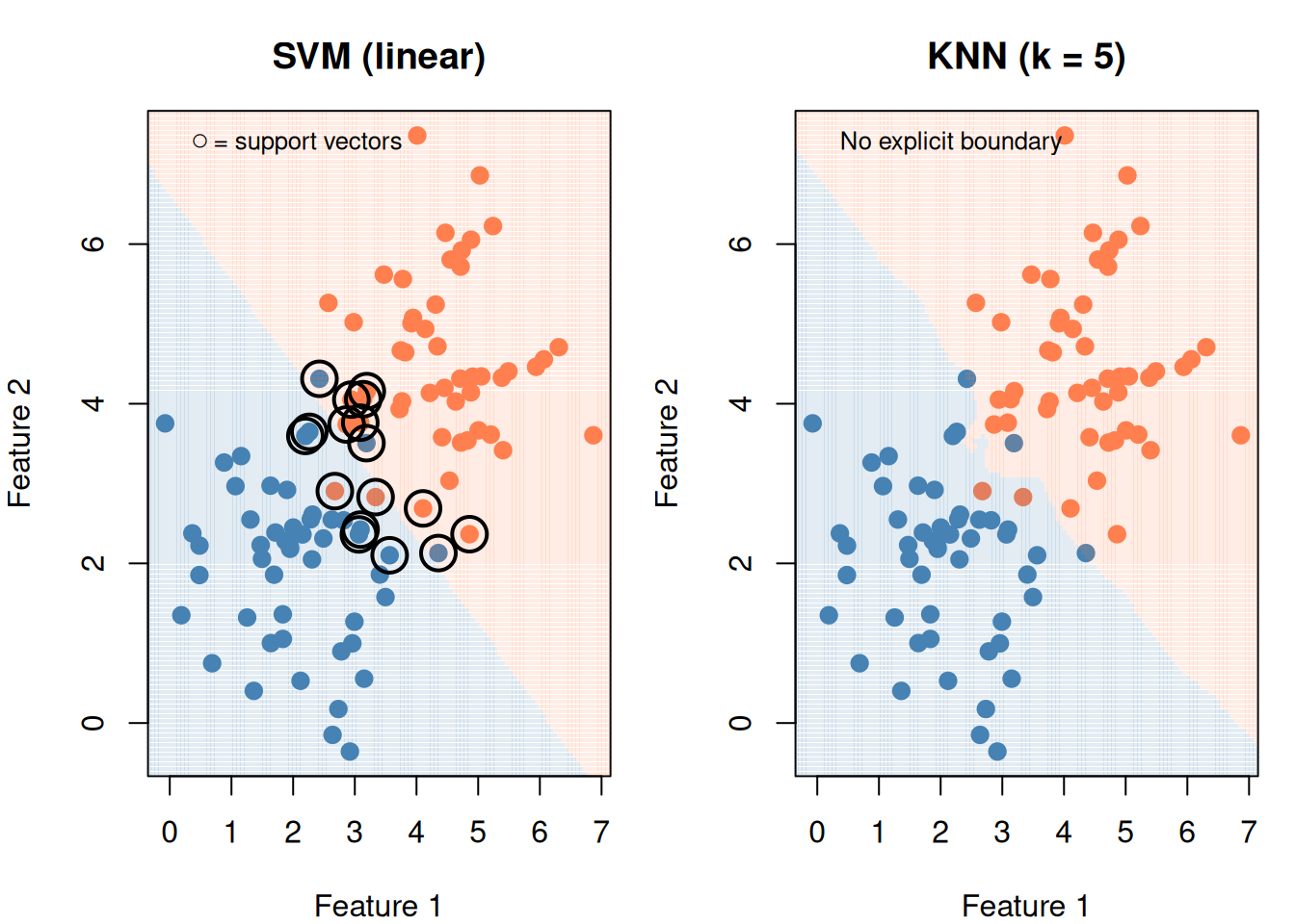
# Slightly overlapping data
set.seed(55)
df_cmp <- data.frame(
  x1 = c(rnorm(50, 2, 1), rnorm(50, 4.5, 1)),
  x2 = c(rnorm(50, 2, 1), rnorm(50, 4.5, 1)),
  group = factor(rep(c("A", "B"), each = 50))
)

grid_cmp <- expand.grid(
  x1 = seq(-1, 8, length.out = 150),
  x2 = seq(-1, 8, length.out = 150)
)

par(mfrow = c(1, 2), mar = c(4, 4, 3, 1))

# SVM
fit_svm <- svm(group ~ x1 + x2, data = df_cmp, kernel = "linear", cost = 1)
grid_cmp$svm_pred <- predict(fit_svm, grid_cmp)

plot(df_cmp$x1, df_cmp$x2,
  col = ifelse(df_cmp$group == "A", "steelblue", "coral"),
  pch = 19, cex = 1.2, main = "SVM (linear)",
  xlab = "Feature 1", ylab = "Feature 2")
points(grid_cmp$x1, grid_cmp$x2,
  col = ifelse(grid_cmp$svm_pred == "A",
    adjustcolor("steelblue", 0.15), adjustcolor("coral", 0.15)),
  pch = 15, cex = 0.3)
points(df_cmp$x1[fit_svm$index], df_cmp$x2[fit_svm$index],
  pch = 1, cex = 2.5, lwd = 2)
legend("topleft", bty = "n", legend = "○ = support vectors", cex = 0.8)

# KNN
knn_pred <- knn(
  train = df_cmp[, c("x1", "x2")],
  test = grid_cmp[, c("x1", "x2")],
  cl = df_cmp$group, k = 5
)

plot(df_cmp$x1, df_cmp$x2,
  col = ifelse(df_cmp$group == "A", "steelblue", "coral"),
  pch = 19, cex = 1.2, main = "KNN (k = 5)",
  xlab = "Feature 1", ylab = "Feature 2")
points(grid_cmp$x1, grid_cmp$x2,
  col = ifelse(knn_pred == "A",
    adjustcolor("steelblue", 0.15), adjustcolor("coral", 0.15)),
  pch = 15, cex = 0.3)
legend("topleft", bty = "n", legend = "No explicit boundary", cex = 0.8)

par(mfrow = c(1, 1))

Figure 9: Same data, different approaches: SVM draws a boundary, KNN uses local voting

9. Strengths and Weaknesses

Strengths

• Dead simple — no training, no assumptions about data shape
• Non-linear for free — the boundary naturally curves around data
• Multi-class for free — just count votes
• No training time — just store the data

Weaknesses (The Curse of Dimensionality)

As the number of features grows, distances become meaningless. In high dimensions, all points are roughly the same distance from each other.

set.seed(1)
dims <- c(2, 5, 10, 50, 100, 500)
ratios <- sapply(dims, function(d) {
  data <- matrix(rnorm(1000 * d), ncol = d)
  query <- rnorm(d)
  dists <- sqrt(rowSums((data - matrix(query, nrow = 1000, ncol = d, byrow = TRUE))^2))
  max(dists) / min(dists)
})

barplot(ratios, names.arg = dims,
  col = "steelblue", border = NA,
  xlab = "Number of Features",
  ylab = "Max Distance / Min Distance",
  main = "Curse of Dimensionality")
abline(h = 1, lty = 2, col = "red")
text(6, 1.3, "ratio → 1 means all distances are similar\n(KNN can't distinguish neighbors)",
     col = "red", cex = 0.8)

Figure 10: In high dimensions, the gap between nearest and farthest neighbor shrinks

Fix: Use PCA (Module 9) to reduce dimensions before applying KNN.

10. Cheat Sheet: The Whole Story on One Page

THE KNN RECIPE
==============

1. ALGORITHM:
   - Compute distance from new point to all training points
   - Find k closest neighbors
   - Classification: majority vote
   - Regression: average of neighbors' values

2. THE FORMULA:

   Euclidean distance:  d = √(Σ(xⱼ - xⱼ')²)
   Prediction:          ŷ = mode of k nearest labels

3. KEY PARAMETER:
   k → number of neighbors  (tune via cross-validation)
     small k = overfit (jagged boundary, memorizes noise)
     large k = underfit (smooth boundary, misses patterns)
     Rule of thumb: start with k = √n

4. MANDATORY: SCALE YOUR FEATURES
   Same reason as SVM — distance-based method

5. STRENGTHS:
   - No training needed (lazy learner)
   - Handles non-linear boundaries naturally
   - Multi-class without modification

6. WEAKNESSES:
   - Slow prediction (computes all distances)
   - Stores entire training set
   - Curse of dimensionality (fails with many features)
   - No model to interpret

11. Check Your Understanding

NoteTest Yourself

Before moving on, try to answer these without scrolling up:

1. In one sentence, what does KNN do?
2. Why is KNN called a “lazy learner”?
3. What happens to the decision boundary when you increase \(k\)? Decrease it?
4. Why is scaling mandatory for KNN?
5. What is the curse of dimensionality and how does it affect KNN?
6. When would you pick KNN over SVM? When would you pick SVM over KNN?
7. How do you choose the best \(k\)? (Hint: not a formula)