k-Means Clustering From Scratch: Finding Groups Nobody Told You About

Unsupervised learning — no labels, no teacher, just patterns

1. The Problem: No Labels

Everything so far — SVM, KNN — assumed you had labeled data. You knew which group each point belonged to, and the goal was to learn the rule.

But what if you have no labels? Nobody told you the groups. You just have a pile of data and a question: are there natural groupings hiding in here?

library(ggplot2)
set.seed(42)

# Three hidden clusters
true_centers <- data.frame(x1 = c(2, 6, 4), x2 = c(2, 2, 6))
n_per <- 60

df <- data.frame(
  x1 = c(rnorm(n_per, 2, 0.7), rnorm(n_per, 6, 0.7), rnorm(n_per, 4, 0.7)),
  x2 = c(rnorm(n_per, 2, 0.7), rnorm(n_per, 2, 0.7), rnorm(n_per, 6, 0.7)),
  true_group = factor(rep(c("A", "B", "C"), each = n_per))
)

# Show without labels
ggplot(df, aes(x1, x2)) +
  geom_point(size = 2, color = "gray30") +
  theme_minimal(base_size = 14) +
  labs(x = "Feature 1", y = "Feature 2",
       title = "All you see: unlabeled points")

Figure 1: You see the data. Can you spot the groups? k-means can.

This is unsupervised learning. No response variable, no “right answer.” The algorithm has to discover structure on its own.

2. The k-Means Algorithm: 4 Steps on Repeat

k-means is embarrassingly simple:

1. Pick \(k\) random starting centers (centroids)
2. Assign each point to the nearest center
3. Move each center to the average of its assigned points
4. Repeat steps 2-3 until nothing changes

That’s the whole algorithm. Let’s watch it happen.

set.seed(15)

# Manual k-means to show each step
k <- 3
centers <- df[sample(nrow(df), k), c("x1", "x2")]
colors <- c("coral", "steelblue", "forestgreen")

par(mfrow = c(2, 3), mar = c(3, 3, 3, 1))

for (iter in 1:6) {
  # Step 2: Assign to nearest center
  dists <- sapply(1:k, function(j) {
    sqrt((df$x1 - centers$x1[j])^2 + (df$x2 - centers$x2[j])^2)
  })
  assignments <- apply(dists, 1, which.min)

  plot(df$x1, df$x2,
    col = adjustcolor(colors[assignments], 0.5),
    pch = 19, cex = 1,
    main = paste("Iteration", iter),
    xlab = "x1", ylab = "x2")

  # Show centers
  points(centers$x1, centers$x2, pch = 4, cex = 3, lwd = 3,
         col = colors[1:k])

  # Draw lines from centers to their points (first iteration only)
  if (iter == 1) {
    legend("topright", bty = "n", cex = 0.7,
      legend = "✕ = cluster centers")
  }

  # Step 3: Move centers
  for (j in 1:k) {
    members <- df[assignments == j, ]
    centers$x1[j] <- mean(members$x1)
    centers$x2[j] <- mean(members$x2)
  }
}
par(mfrow = c(1, 1))

Figure 2: k-means in action: assign → move centers → assign → move → converge

After a few iterations, the centers stop moving — the algorithm has converged. Each point belongs to the cluster whose center is closest.

3. The Formula: What k-Means Minimizes

k-means minimizes the total within-cluster sum of squares (WCSS):

\[\min \sum_{j=1}^{k} \sum_{\mathbf{x}_i \in C_j} \|\mathbf{x}_i - \boldsymbol{\mu}_j\|^2\]

Let’s unpack every piece:

Symbol	What it is	Plain English
\(k\)	Number of clusters	How many groups you want
\(C_j\)	Cluster \(j\)	The set of points assigned to group \(j\)
\(\mathbf{x}_i\)	A data point	One observation
\(\boldsymbol{\mu}_j\)	Center (centroid) of cluster \(j\)	The average of all points in group \(j\)
\(\|\mathbf{x}_i - \boldsymbol{\mu}_j\|^2\)	Squared distance	How far point \(i\) is from its cluster center

In plain English: make each point as close as possible to the center of its assigned cluster. Tight clusters = low WCSS = good.

# Final k-means result
km <- kmeans(df[, c("x1", "x2")], centers = 3, nstart = 20)

df$cluster <- factor(km$cluster)
centers_final <- as.data.frame(km$centers)
centers_final$cluster <- factor(1:3)

ggplot(df, aes(x1, x2, color = cluster)) +
  geom_segment(aes(xend = km$centers[as.numeric(cluster), 1],
                    yend = km$centers[as.numeric(cluster), 2]),
               alpha = 0.15, linewidth = 0.3) +
  geom_point(size = 2) +
  geom_point(data = centers_final, aes(x1, x2),
             shape = 4, size = 5, stroke = 3, color = "black") +
  scale_color_manual(values = c("coral", "steelblue", "forestgreen")) +
  theme_minimal(base_size = 14) +
  labs(x = "Feature 1", y = "Feature 2",
       title = paste("Total WCSS =", round(km$tot.withinss, 1)),
       subtitle = "Each line = distance from point to its center") +
  theme(legend.position = "none")

Figure 3: WCSS = sum of all these distances (squared). k-means tries to make this small.

The Centroid Formula

The center of cluster \(j\) is simply the mean of all points assigned to it:

\[\boldsymbol{\mu}_j = \frac{1}{|C_j|} \sum_{\mathbf{x}_i \in C_j} \mathbf{x}_i\]

That’s why it’s called k-means — the centers are the means of their clusters.

4. The Assignment Rule: Nearest Center

Each point goes to the cluster whose center is closest (Euclidean distance):

\[\text{cluster}(\mathbf{x}_i) = \arg\min_j \|\mathbf{x}_i - \boldsymbol{\mu}_j\|^2\]

This is the same distance formula from KNN. The difference: KNN looks at nearest data points. k-means looks at nearest cluster centers.

# Show decision regions
grid <- expand.grid(
  x1 = seq(min(df$x1) - 1, max(df$x1) + 1, length.out = 200),
  x2 = seq(min(df$x2) - 1, max(df$x2) + 1, length.out = 200)
)

dists_grid <- sapply(1:3, function(j) {
  sqrt((grid$x1 - km$centers[j, 1])^2 + (grid$x2 - km$centers[j, 2])^2)
})
grid$cluster <- factor(apply(dists_grid, 1, which.min))

ggplot() +
  geom_tile(data = grid, aes(x1, x2, fill = cluster), alpha = 0.15) +
  geom_point(data = df, aes(x1, x2, color = cluster), size = 2) +
  geom_point(data = centers_final, aes(x1, x2),
             shape = 4, size = 5, stroke = 3, color = "black") +
  scale_fill_manual(values = c("coral", "steelblue", "forestgreen")) +
  scale_color_manual(values = c("coral", "steelblue", "forestgreen")) +
  theme_minimal(base_size = 14) +
  labs(x = "Feature 1", y = "Feature 2",
       title = "Cluster territories: every location maps to its nearest center") +
  theme(legend.position = "none")

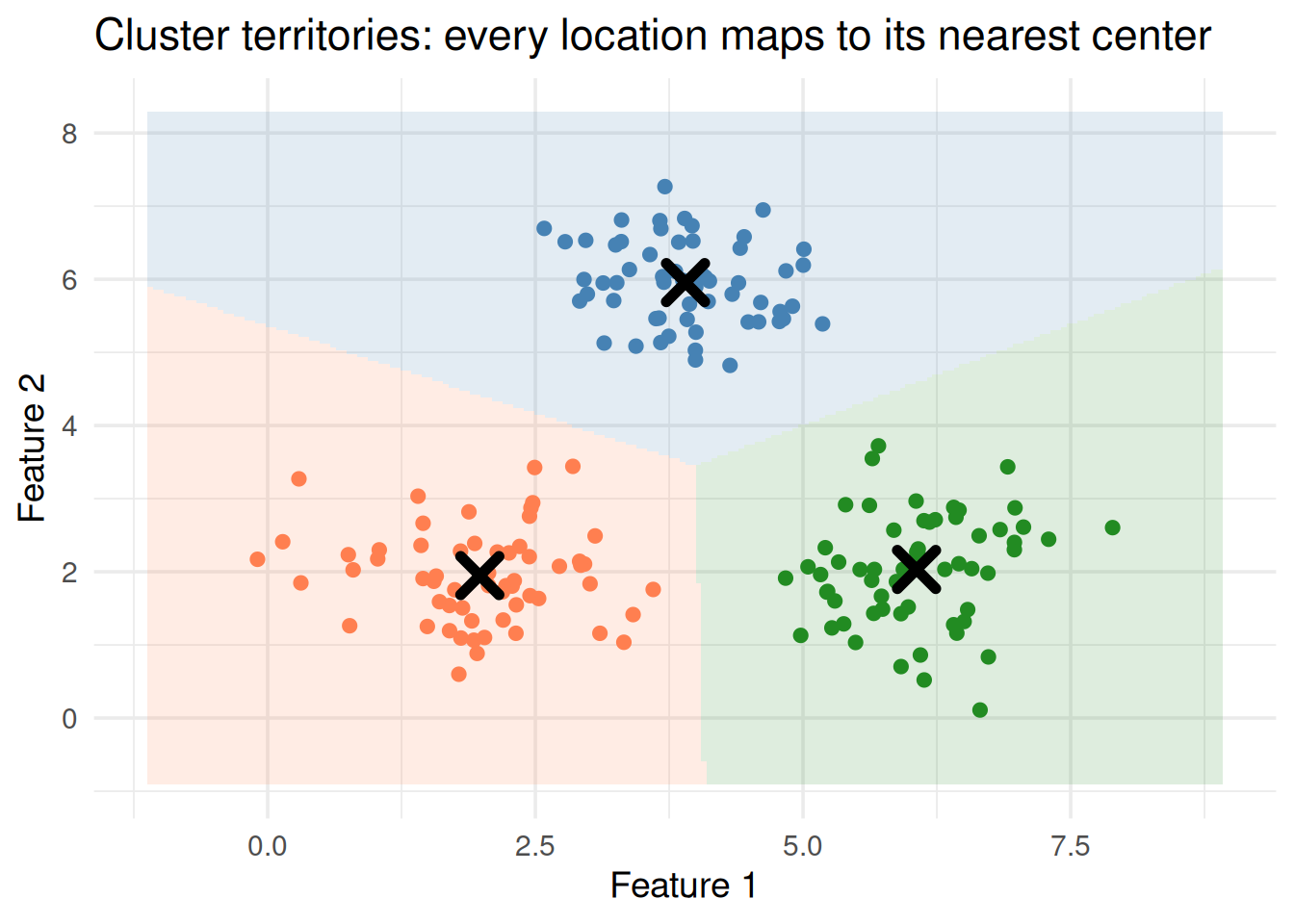
Figure 4: Each region contains all points closest to that center (Voronoi diagram)

5. Choosing k: The Elbow Method

The hardest part of k-means: how many clusters? There’s no formula. You use the elbow method:

1. Run k-means for \(k = 1, 2, 3, \dots\)
2. Record the total WCSS for each \(k\)
3. Plot \(k\) vs WCSS
4. Look for the elbow — where the curve bends and adding more clusters stops helping much

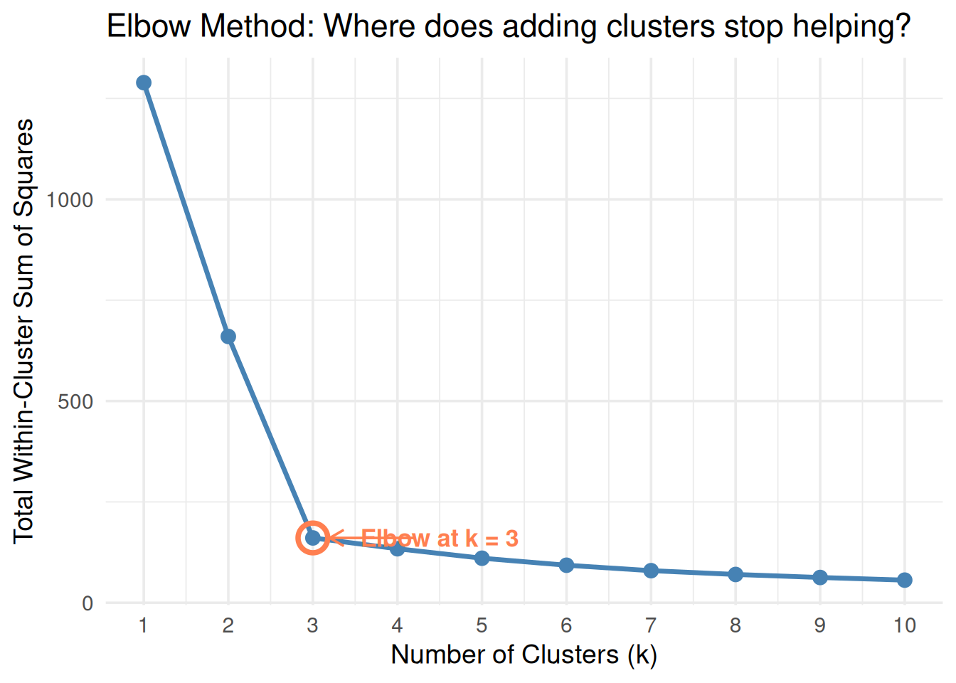
k_range <- 1:10
wcss <- sapply(k_range, function(k) {
  km_fit <- kmeans(df[, c("x1", "x2")], centers = k, nstart = 20)
  km_fit$tot.withinss
})

elbow_df <- data.frame(k = k_range, wcss = wcss)

ggplot(elbow_df, aes(k, wcss)) +
  geom_line(linewidth = 1.2, color = "steelblue") +
  geom_point(size = 3, color = "steelblue") +
  geom_point(data = elbow_df[3, ], aes(k, wcss),
             size = 6, shape = 1, color = "coral", stroke = 2) +
  annotate("text", x = 4.5, y = wcss[3],
           label = "Elbow at k = 3", color = "coral", size = 4.5, fontface = "bold") +
  annotate("segment", x = 4.2, xend = 3.2, y = wcss[3], yend = wcss[3],
           arrow = arrow(length = unit(0.3, "cm")), color = "coral") +
  scale_x_continuous(breaks = k_range) +
  theme_minimal(base_size = 14) +
  labs(x = "Number of Clusters (k)", y = "Total Within-Cluster Sum of Squares",
       title = "Elbow Method: Where does adding clusters stop helping?")

Figure 5: The elbow method: WCSS drops sharply, then flattens — the bend is your k

Why \(k = 3\) here? Going from 2 to 3 clusters gives a big drop in WCSS. Going from 3 to 4 gives almost nothing. The “elbow” bends at 3.

Important: The elbow is a judgment call, not an exact calculation. Sometimes the elbow is obvious; sometimes it’s ambiguous. In this guide, the setup will make it clear.

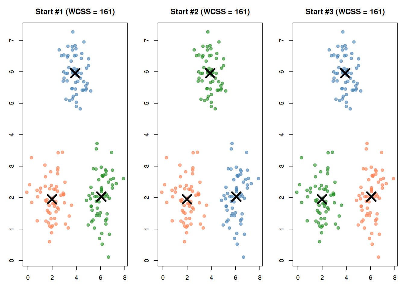
6. The Random Initialization Problem

k-means starts with random centers. Different starting positions can lead to different results — sometimes bad ones.

par(mfrow = c(1, 3), mar = c(3, 3, 3, 1))

colors <- c("coral", "steelblue", "forestgreen")

for (trial in c(1, 2, 3)) {
  set.seed(trial * 7)
  km_trial <- kmeans(df[, c("x1", "x2")], centers = 3, nstart = 1)

  plot(df$x1, df$x2,
    col = adjustcolor(colors[km_trial$cluster], 0.6),
    pch = 19, cex = 1,
    main = paste0("Start #", trial, " (WCSS = ", round(km_trial$tot.withinss, 0), ")"),
    xlab = "x1", ylab = "x2")
  points(km_trial$centers[, 1], km_trial$centers[, 2],
         pch = 4, cex = 3, lwd = 3)
}
par(mfrow = c(1, 1))

Figure 6: Same data, same k=3, but different random starts → different results

The fix: Run k-means many times with different random starts and keep the result with the lowest WCSS.

In R: kmeans(data, centers = k, nstart = 20) runs it 20 times automatically.

nstart_vals <- c(1, 5, 10, 25, 50)
best_wcss <- sapply(nstart_vals, function(ns) {
  results <- replicate(20, {
    km_fit <- kmeans(df[, c("x1", "x2")], centers = 3, nstart = ns)
    km_fit$tot.withinss
  })
  mean(results)
})

ggplot(data.frame(nstart = nstart_vals, wcss = best_wcss), aes(nstart, wcss)) +
  geom_line(linewidth = 1, color = "steelblue") +
  geom_point(size = 3, color = "steelblue") +
  theme_minimal(base_size = 14) +
  labs(x = "nstart (number of random starts)", y = "Average WCSS found",
       title = "More starts = better solution (diminishing returns past ~20)")

Figure 7: More random starts → more likely to find the best clustering

7. Why Scaling Is Mandatory (Again)

Same story as KNN and SVM. k-means uses distance. Unscaled features with large ranges dominate.

set.seed(42)

# Customer data: income (30k-90k) and age (18-70)
customers <- data.frame(
  income = c(rnorm(40, 40000, 5000), rnorm(40, 75000, 5000)),
  age = c(rnorm(40, 25, 4), rnorm(40, 55, 4))
)

par(mfrow = c(1, 2), mar = c(4, 4, 3, 1))

# Unscaled
km_raw <- kmeans(customers, 2, nstart = 20)
plot(customers$income, customers$age,
  col = c("coral", "steelblue")[km_raw$cluster],
  pch = 19, main = "Unscaled: income dominates",
  xlab = "Income ($)", ylab = "Age")

# Scaled
cust_scaled <- scale(customers)
km_scaled <- kmeans(cust_scaled, 2, nstart = 20)
plot(customers$income, customers$age,
  col = c("coral", "steelblue")[km_scaled$cluster],
  pch = 19, main = "Scaled: both features contribute",
  xlab = "Income ($)", ylab = "Age")

par(mfrow = c(1, 1))

Figure 8: Without scaling, the high-range feature dominates cluster assignments

8. Supervised vs Unsupervised: The Big Picture

This is an high-value distinction. Know the difference cold.

	Supervised (SVM, KNN)	Unsupervised (k-means)
Labels?	Yes — you know the groups	No — groups are unknown
Goal	Learn the rule to predict labels	Discover hidden structure
Evaluation	Accuracy, cross-validation	WCSS, silhouette, elbow method
k means…	(KNN) number of neighbors	(k-means) number of clusters
Example	“Is this email spam?”	“What types of customers do we have?”

par(mfrow = c(1, 2), mar = c(4, 4, 3, 1))

# Supervised: labeled data with boundary
plot(df$x1, df$x2,
  col = c("coral", "steelblue", "forestgreen")[as.numeric(df$true_group)],
  pch = 19, cex = 1.2,
  main = "Supervised: labels given",
  xlab = "Feature 1", ylab = "Feature 2")
legend("topleft", legend = c("A", "B", "C"), bty = "n",
  col = c("coral", "steelblue", "forestgreen"), pch = 19, cex = 0.8,
  title = "Known labels")

# Unsupervised: same data, no labels, discover clusters
plot(df$x1, df$x2,
  col = c("coral", "steelblue", "forestgreen")[km$cluster],
  pch = 19, cex = 1.2,
  main = "Unsupervised: clusters discovered",
  xlab = "Feature 1", ylab = "Feature 2")
points(km$centers[, 1], km$centers[, 2], pch = 4, cex = 3, lwd = 3)
legend("topleft", legend = paste("Cluster", 1:3), bty = "n",
  col = c("coral", "steelblue", "forestgreen"), pch = 19, cex = 0.8,
  title = "Discovered groups")

par(mfrow = c(1, 1))

Figure 9: Left: supervised (labels known, learn boundary). Right: unsupervised (no labels, find groups).

9. k-Means Limitations

It assumes spherical clusters

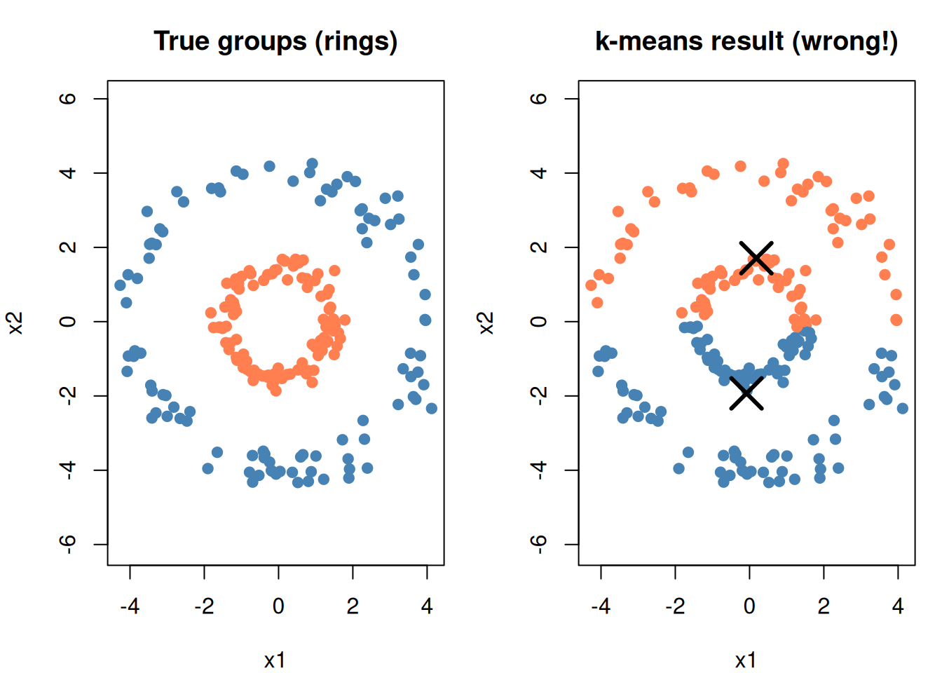
k-means draws boundaries equidistant from centers — producing circular (spherical) regions. Data with elongated, curved, or irregular shapes won’t cluster well.

set.seed(42)

# Concentric rings (k-means will fail)
n <- 200
angle <- runif(n, 0, 2 * pi)
r_inner <- rnorm(n / 2, 1.5, 0.2)
r_outer <- rnorm(n / 2, 4, 0.3)

rings <- data.frame(
  x1 = c(r_inner * cos(angle[1:(n/2)]), r_outer * cos(angle[(n/2+1):n])),
  x2 = c(r_inner * sin(angle[1:(n/2)]), r_outer * sin(angle[(n/2+1):n])),
  true = factor(rep(c("Inner", "Outer"), each = n / 2))
)

km_rings <- kmeans(rings[, 1:2], 2, nstart = 20)

par(mfrow = c(1, 2), mar = c(4, 4, 3, 1))

plot(rings$x1, rings$x2,
  col = c("coral", "steelblue")[as.numeric(rings$true)],
  pch = 19, main = "True groups (rings)",
  xlab = "x1", ylab = "x2", asp = 1)

plot(rings$x1, rings$x2,
  col = c("coral", "steelblue")[km_rings$cluster],
  pch = 19, main = "k-means result (wrong!)",
  xlab = "x1", ylab = "x2", asp = 1)
points(km_rings$centers[, 1], km_rings$centers[, 2],
       pch = 4, cex = 3, lwd = 3)

par(mfrow = c(1, 1))

Figure 10: k-means struggles with non-spherical shapes

Other limitations

• You must choose k in advance — the algorithm can’t decide for you
• Sensitive to outliers — a single extreme point can pull a center away
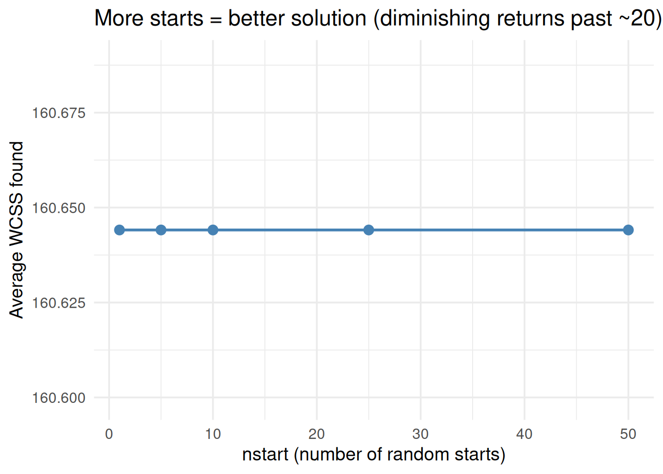
• Random starts — can get stuck in bad solutions (fix: use nstart)
• Only finds convex clusters — can’t wrap around shapes

10. Practical Use: Customer Segmentation

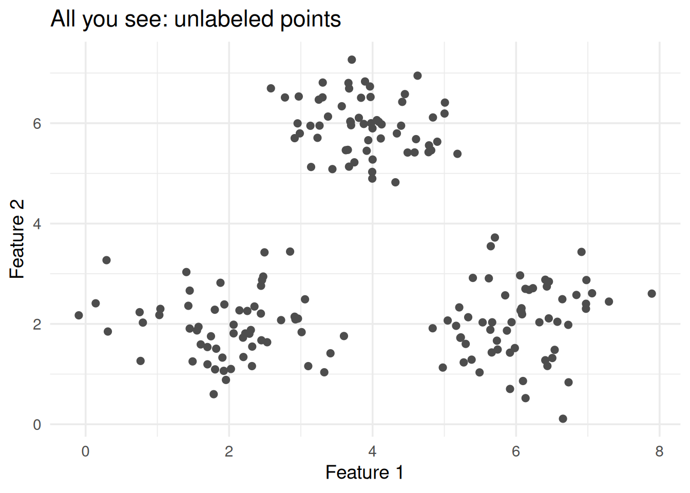
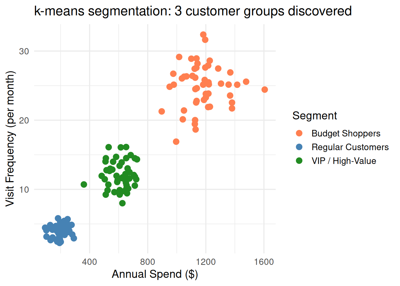
This is the classic practice scenario. You have customer data, no labels, and the business wants to know: what types of customers do we have?

set.seed(42)

# Simulated customer data
customers2 <- data.frame(
  annual_spend = c(rnorm(50, 200, 40), rnorm(50, 600, 80), rnorm(50, 1200, 150)),
  visit_frequency = c(rnorm(50, 4, 1), rnorm(50, 12, 2), rnorm(50, 25, 3))
)

# Scale then cluster
cust_s <- scale(customers2)
km_cust <- kmeans(cust_s, 3, nstart = 20)

customers2$segment <- factor(km_cust$cluster)

# Label segments meaningfully
seg_means <- aggregate(cbind(annual_spend, visit_frequency) ~ segment, data = customers2, mean)
seg_means <- seg_means[order(seg_means$annual_spend), ]
seg_labels <- c("Budget Shoppers", "Regular Customers", "VIP / High-Value")

ggplot(customers2, aes(annual_spend, visit_frequency, color = segment)) +
  geom_point(size = 3) +
  scale_color_manual(values = c("coral", "steelblue", "forestgreen"),
                     labels = seg_labels) +
  theme_minimal(base_size = 14) +
  labs(x = "Annual Spend ($)", y = "Visit Frequency (per month)",
       color = "Segment",
       title = "k-means segmentation: 3 customer groups discovered")

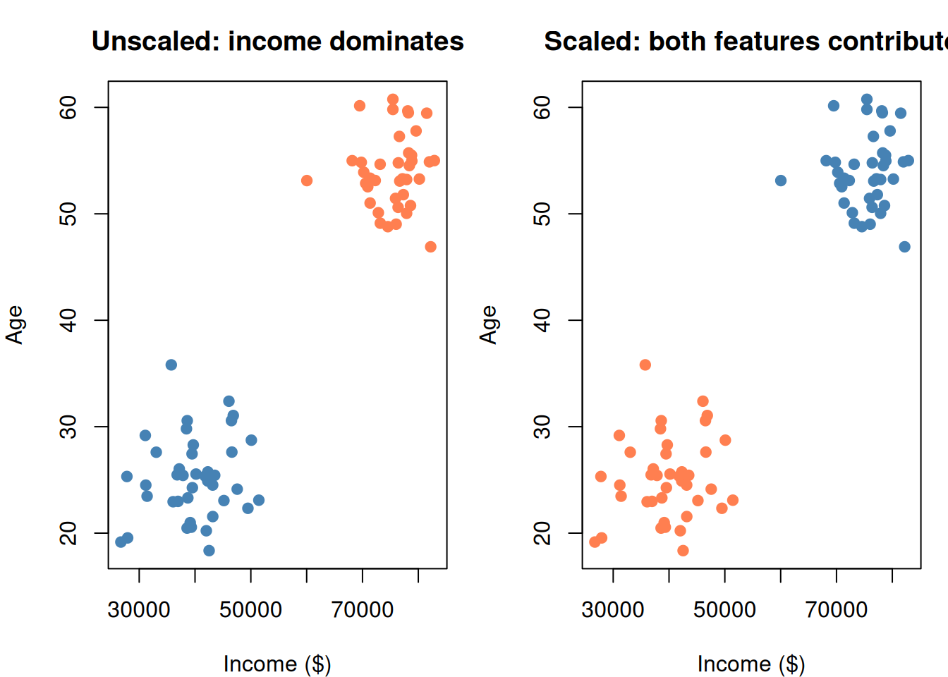
Figure 11: Customer segmentation: k-means discovers 3 natural groups from spending data

The workflow:

1. Collect customer features (spend, visits, demographics, etc.)
2. Scale the features
3. Use elbow method to choose \(k\)
4. Run k-means with nstart = 20
5. Interpret the clusters → give them business-meaningful names
6. Build different strategies per segment

11. Cheat Sheet: The Whole Story on One Page

THE k-MEANS RECIPE
===================

1. ALGORITHM (repeat until convergence):
   - Assign each point to nearest center
   - Move each center to mean of its points

2. THE FORMULA:

   min  Σⱼ Σᵢ∈Cⱼ ||xᵢ - μⱼ||²
        -------------------------
        "total distance from points
         to their cluster centers"

   Center of cluster j:  μⱼ = (1/|Cⱼ|) × Σ xᵢ

3. KEY PARAMETER:
   k → number of clusters (choose via elbow method)

4. ELBOW METHOD:
   Plot k vs WCSS → pick the "bend" point

5. GOTCHAS:
   - Random initialization → use nstart = 20
   - ALWAYS scale features first
   - Assumes spherical clusters
   - You must choose k in advance

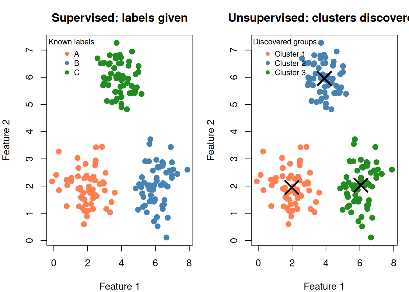
6. SUPERVISED vs UNSUPERVISED:
   Labels → supervised (SVM, KNN)
   No labels → unsupervised (k-means)

7. PRACTICE TIP:
   "Segment customers" / "find groups" / "no labels" → k-means
   "Classify" / "predict category" / "labeled data" → SVM, KNN

12. Check Your Understanding

NoteTest Yourself

Before moving on, try to answer these without scrolling up:

1. What makes k-means unsupervised? How is this different from KNN?
2. Describe the k-means algorithm in 4 steps.
3. What does k-means minimize? Write the formula in words.
4. Why is the centroid the mean of the cluster points?
5. How does the elbow method work? What are you plotting?
6. Why do you need to run k-means with multiple random starts?
7. Give a scenario where k-means would fail. Why does it fail?
8. A question says “we have customer purchase data and want to identify different customer types.” Which model? Why not SVM?