PCA & Box-Cox From Scratch: Fixing Your Data Before Modeling

Dimensionality reduction and variance stabilization

1. The Problem: Too Many Correlated Predictors

You’re building a regression model. You have 50 predictors. Many of them measure similar things — they’re correlated. This causes problems:

• Multicollinearity: correlated predictors make coefficients unstable
• Overfitting: too many predictors relative to data points
• Noise: some predictors are mostly noise, not signal

PCA solves all three by compressing your predictors into a smaller set of uncorrelated components that capture the important patterns.

library(ggplot2)
set.seed(42)

n <- 100

# Two correlated features
x1 <- rnorm(n, 50, 10)
x2 <- 0.8 * x1 + rnorm(n, 10, 5)  # correlated with x1

df <- data.frame(x1 = x1, x2 = x2)

ggplot(df, aes(x1, x2)) +
  geom_point(size = 2, color = "gray40") +
  theme_minimal(base_size = 14) +
  labs(x = "Feature 1 (e.g., assessment score)",
       y = "Feature 2 (e.g., homework score)",
       title = paste0("Correlation = ", round(cor(x1, x2), 2),
                       " — these carry overlapping information"))

Figure 1: These two features are highly correlated — they carry redundant information

If both features carry almost the same information, do you really need both? PCA finds the directions in the data that capture the most variation, and lets you keep just those.

2. PCA: What It Does Geometrically

PCA rotates your coordinate system so that:

1. The first axis (PC1) points in the direction of maximum spread
2. The second axis (PC2) points perpendicular to PC1, capturing the next most spread
3. And so on…

# Standardize
df_s <- scale(df)

# PCA
pca <- prcomp(df_s)

# Plot original data with PCA directions
par(mfrow = c(1, 2), mar = c(4, 4, 3, 1))

# Original space with PCA arrows
plot(df_s[, 1], df_s[, 2], pch = 19, col = "gray40", asp = 1,
  main = "Original Space + PCA Directions",
  xlab = "Feature 1 (standardized)", ylab = "Feature 2 (standardized)")

# PC1 direction
arrows(0, 0, pca$rotation[1, 1] * 2, pca$rotation[2, 1] * 2,
  col = "coral", lwd = 3, length = 0.15)
text(pca$rotation[1, 1] * 2.3, pca$rotation[2, 1] * 2.3,
  "PC1", col = "coral", font = 2, cex = 1.2)

# PC2 direction
arrows(0, 0, pca$rotation[1, 2] * 1.5, pca$rotation[2, 2] * 1.5,
  col = "steelblue", lwd = 3, length = 0.15)
text(pca$rotation[1, 2] * 1.8, pca$rotation[2, 2] * 1.8,
  "PC2", col = "steelblue", font = 2, cex = 1.2)

# Rotated space (PCA scores)
scores <- pca$x
plot(scores[, 1], scores[, 2], pch = 19, col = "gray40", asp = 1,
  main = "PCA Space (Rotated)",
  xlab = "PC1 (most variance)", ylab = "PC2 (remaining variance)")
abline(h = 0, v = 0, lty = 2, col = "gray70")

par(mfrow = c(1, 1))

Figure 2: PCA rotates the axes to align with the directions of maximum variance

Notice in the PCA space:

• PC1 (horizontal) captures the main spread — most of the information
• PC2 (vertical) captures what’s left — much less spread
• The two components are uncorrelated (perpendicular)

3. The PCA Algorithm: Step by Step

1. Standardize the data (mean = 0, SD = 1 for each feature)
2. Compute the covariance matrix (\(\mathbf{X}^T \mathbf{X}\))
3. Find the eigenvalues and eigenvectors
4. Sort by eigenvalue (largest first)
5. First eigenvector = PC1, second = PC2, etc.

What Are Eigenvalues and Eigenvectors?

Concept	What it is	Plain English
Eigenvector	A direction in feature space	Which way does the data spread?
Eigenvalue	A number paired with each eigenvector	How much variance is in that direction?

The eigenvector with the largest eigenvalue points in the direction of maximum variance — that’s PC1.

# Show eigenvalues
eigenvalues <- pca$sdev^2
var_explained <- eigenvalues / sum(eigenvalues) * 100

cat("Eigenvalues:\n")

Eigenvalues:

cat(sprintf("  PC1: %.2f (%.1f%% of variance)\n", eigenvalues[1], var_explained[1]))

  PC1: 1.88 (94.1% of variance)

cat(sprintf("  PC2: %.2f (%.1f%% of variance)\n", eigenvalues[2], var_explained[2]))

  PC2: 0.12 (5.9% of variance)

cat(sprintf("\nPC1 alone captures %.1f%% of the information!\n", var_explained[1]))

PC1 alone captures 94.1% of the information!

cat("With correlated data, you can often drop PC2 and lose very little.")

With correlated data, you can often drop PC2 and lose very little.

4. Higher Dimensions: Where PCA Really Shines

Two features is easy to visualize. But the real power of PCA is compressing many features into a few components.

set.seed(42)

# Generate 10 correlated features (all driven by 2 hidden factors)
hidden1 <- rnorm(n)
hidden2 <- rnorm(n)

features <- matrix(nrow = n, ncol = 10)
for (j in 1:10) {
  w1 <- runif(1, 0.5, 1.5) * sample(c(-1, 1), 1)
  w2 <- runif(1, 0.2, 0.8) * sample(c(-1, 1), 1)
  features[, j] <- w1 * hidden1 + w2 * hidden2 + rnorm(n, 0, 0.5)
}
colnames(features) <- paste0("X", 1:10)

# PCA
pca10 <- prcomp(scale(features))
var_exp10 <- pca10$sdev^2 / sum(pca10$sdev^2) * 100
cum_var <- cumsum(var_exp10)

par(mfrow = c(1, 2), mar = c(4, 4, 3, 1))

# Scree plot
barplot(var_exp10, names.arg = paste0("PC", 1:10),
  col = ifelse(cum_var <= 90, "steelblue", "gray80"),
  main = "Scree Plot: Variance per Component",
  ylab = "% Variance Explained", las = 2)

# Cumulative variance
plot(1:10, cum_var, type = "b", pch = 19, col = "steelblue", lwd = 2,
  main = "Cumulative Variance Explained",
  xlab = "Number of Components", ylab = "% Total Variance",
  ylim = c(0, 100))
abline(h = 90, lty = 2, col = "coral")
text(7, 85, "90% threshold", col = "coral", cex = 0.9)

# Mark how many needed for 90%
n_for_90 <- which(cum_var >= 90)[1]
points(n_for_90, cum_var[n_for_90], pch = 19, cex = 2, col = "coral")
text(n_for_90 + 1, cum_var[n_for_90] - 5,
  paste0(n_for_90, " components\nfor 90%"), col = "coral", cex = 0.9)

par(mfrow = c(1, 1))

Figure 3: 10 correlated features compressed into components — most variance in first 2-3

10 features → 4 components that capture 90%+ of the information. The remaining components are mostly noise.

5. Choosing How Many Components: The Scree Plot / Elbow

Same idea as the elbow method for k-means:

1. Plot eigenvalues (or % variance) for each component
2. Look for the elbow — where the curve flattens
3. Keep components before the dropoff

Alternative rule: Keep components until you reach 80-90% cumulative variance explained.

plot(1:10, pca10$sdev^2, type = "b", pch = 19, col = "steelblue", lwd = 2,
  main = "Scree Plot: Look for the Elbow",
  xlab = "Component Number", ylab = "Eigenvalue")

# Highlight the elbow
points(3, pca10$sdev[3]^2, pch = 1, cex = 3, col = "coral", lwd = 2)
text(4.5, pca10$sdev[3]^2, "Elbow here →\nkeep 2-3 components",
  col = "coral", cex = 0.9)

Figure 4: The scree plot elbow suggests 2-3 components are sufficient

6. The Critical PCA Trap (High-Value Distinction)

WarningPCA Ranks by Variance, NOT Predictive Power

PCA ranks components by variance in X, NOT by predictive power for Y.

A high-variance component might be irrelevant noise. A low-variance component might contain the actual signal you need for prediction.

set.seed(42)

# Create data where the signal is in a low-variance direction
n_trap <- 150
noise_big <- rnorm(n_trap, 0, 5)    # big variance, no signal
noise_med <- rnorm(n_trap, 0, 3)    # medium variance, no signal
signal <- rnorm(n_trap, 0, 1)       # small variance, IS the signal

X_trap <- cbind(
  noise_big + 0.1 * signal,
  noise_med + 0.05 * signal,
  0.5 * noise_big + 0.8 * signal    # signal mixed in
)

y_trap <- 3 * signal + rnorm(n_trap, 0, 0.5)  # y depends on the hidden signal

pca_trap <- prcomp(scale(X_trap))

# Correlation of each PC with y
pc_cor <- sapply(1:3, function(j) cor(pca_trap$x[, j], y_trap))

par(mfrow = c(1, 2), mar = c(4, 4, 3, 1))

barplot(pca_trap$sdev^2, names.arg = paste0("PC", 1:3),
  col = "steelblue", main = "Variance (what PCA ranks by)",
  ylab = "Eigenvalue")

barplot(abs(pc_cor), names.arg = paste0("PC", 1:3),
  col = c("gray70", "gray70", "coral"),
  main = "Correlation with Y (what matters!)",
  ylab = "|Correlation with response|")

par(mfrow = c(1, 1))

cat("PC1 has the MOST variance but the LEAST predictive power.\n")

PC1 has the MOST variance but the LEAST predictive power.

cat("PC3 has the LEAST variance but the MOST predictive power.\n")

PC3 has the LEAST variance but the MOST predictive power.

cat("\nThis is why you MUST validate PCA-based models on actual prediction.\n")

This is why you MUST validate PCA-based models on actual prediction.

cat("Don't blindly drop low-variance components!")

Don't blindly drop low-variance components!

Figure 5: PC1 has the most variance but PC3 actually predicts the response

WarningPractical Rule

PCA is a preprocessing step. You must still validate the full model (PCA + regression/SVM/etc.) via cross-validation.

7. PCA Requirements

Requirement	Why	What happens if violated
Standardize first	Features with larger ranges dominate	PCA reflects scale, not importance
Continuous features	PCA assumes linear relationships	Binary/categorical features need other methods
Some correlation	If features are uncorrelated, PCA can’t compress	You get back the same features

set.seed(42)

# Income: 30k-90k, Age: 20-65
data_unscaled <- data.frame(
  income = rnorm(80, 60000, 15000),
  age = rnorm(80, 40, 10)
)

pca_unscaled <- prcomp(data_unscaled, scale. = FALSE)
pca_scaled <- prcomp(data_unscaled, scale. = TRUE)

par(mfrow = c(1, 2), mar = c(4, 4, 3, 1))

# Loadings comparison
barplot(abs(pca_unscaled$rotation[, 1]), names.arg = c("Income", "Age"),
  col = c("coral", "steelblue"), main = "PC1 Loadings: UNSCALED",
  ylab = "Absolute Loading")
mtext("Income dominates (larger range)", side = 1, line = 2.5, cex = 0.8, col = "red")

barplot(abs(pca_scaled$rotation[, 1]), names.arg = c("Income", "Age"),
  col = c("coral", "steelblue"), main = "PC1 Loadings: SCALED",
  ylab = "Absolute Loading")
mtext("Both contribute fairly", side = 1, line = 2.5, cex = 0.8, col = "darkgreen")

par(mfrow = c(1, 1))

Figure 6: Without scaling, the high-range feature dominates PC1

---

Part 2: Box-Cox Transformation

8. A Different Problem: Unequal Variance

Regression assumes constant variance — the spread of residuals should be the same everywhere. But real data often violates this:

set.seed(42)
x_bc <- runif(100, 1, 20)
y_bc <- 2 * x_bc + rnorm(100, 0, x_bc * 0.8)  # variance grows with x

df_bc <- data.frame(x = x_bc, y = y_bc)
fit_bc <- lm(y ~ x, data = df_bc)

par(mfrow = c(1, 2), mar = c(4, 4, 3, 1))

plot(df_bc$x, df_bc$y, pch = 19, col = "gray40",
  main = "Data: Variance Grows with X",
  xlab = "X", ylab = "Y")
abline(fit_bc, col = "steelblue", lwd = 2)

plot(fitted(fit_bc), residuals(fit_bc), pch = 19, col = "gray40",
  main = "Residual Plot: Funnel Shape",
  xlab = "Fitted Values", ylab = "Residuals")
abline(h = 0, lty = 2, col = "coral")
text(25, 15, "Variance increases →\n(heteroscedasticity)", col = "coral", cex = 0.9)

par(mfrow = c(1, 1))

Figure 7: The funnel shape: variance increases with the predicted value

This funnel shape means the model’s predictions are unreliable — accurate for small values, wildly off for large values.

Box-Cox fixes this by transforming the response variable.

9. The Box-Cox Formula

\[T(y) = \begin{cases} \frac{y^{\lambda} - 1}{\lambda} & \text{if } \lambda \neq 0 \\ \log(y) & \text{if } \lambda = 0 \end{cases}\]

Symbol	What it is	Plain English
\(y\)	Original response variable	The thing you’re predicting
\(T(y)\)	Transformed response	The stabilized version
\(\lambda\)	Power parameter	Controls the shape of the transformation

Special cases of \(\lambda\):

\(\lambda\)	Transform	Effect
1	\(y\) (no change)	Data is fine as-is
0.5	\(\sqrt{y}\)	Mild compression of large values
0	\(\log(y)\)	Strong compression — common in practice
-1	\(1/y\)	Very aggressive compression

Box-Cox finds the optimal \(\lambda\) automatically by trying different values and picking the one that makes the residuals most normally distributed.

library(MASS)

# Need positive y for Box-Cox
y_pos <- y_bc - min(y_bc) + 1
df_pos <- data.frame(x = x_bc, y = y_pos)
fit_pos <- lm(y ~ x, data = df_pos)

# Box-Cox profile
bc <- boxcox(fit_pos, plotit = TRUE)

# Find optimal lambda
optimal_lambda <- bc$x[which.max(bc$y)]
cat(sprintf("\nOptimal λ = %.2f\n", optimal_lambda))

Optimal λ = 0.55

cat(sprintf("Closest standard transform: %s\n",
  ifelse(abs(optimal_lambda) < 0.2, "log(y)",
    ifelse(abs(optimal_lambda - 0.5) < 0.2, "√y",
      ifelse(abs(optimal_lambda - 1) < 0.2, "no transform needed",
        paste0("y^", round(optimal_lambda, 2)))))))

Closest standard transform: √y

Figure 8: Box-Cox finds the optimal λ that stabilizes variance

# Apply transform
if (abs(optimal_lambda) < 0.01) {
  y_transformed <- log(y_pos)
} else {
  y_transformed <- (y_pos^optimal_lambda - 1) / optimal_lambda
}

df_trans <- data.frame(x = x_bc, y = y_transformed)
fit_trans <- lm(y ~ x, data = df_trans)

par(mfrow = c(2, 2), mar = c(4, 4, 3, 1))

# Before
plot(fitted(fit_pos), residuals(fit_pos), pch = 19, col = "coral",
  main = "BEFORE Box-Cox: Residuals",
  xlab = "Fitted", ylab = "Residual")
abline(h = 0, lty = 2)

hist(residuals(fit_pos), breaks = 15, col = "coral", border = "white",
  main = "BEFORE: Residual Distribution", xlab = "Residual")

# After
plot(fitted(fit_trans), residuals(fit_trans), pch = 19, col = "steelblue",
  main = "AFTER Box-Cox: Residuals",
  xlab = "Fitted", ylab = "Residual")
abline(h = 0, lty = 2)

hist(residuals(fit_trans), breaks = 15, col = "steelblue", border = "white",
  main = "AFTER: Residual Distribution", xlab = "Residual")

par(mfrow = c(1, 1))

Figure 9: Before and after Box-Cox: the funnel shape disappears

The funnel shape is gone. Residuals are more uniform and more normal.

10. Detrending: Removing Time’s Influence

When you want to study the relationship between X and Y, but both are trending over time, the time trend creates a spurious correlation.

Fix: Remove the trend first, then analyze the detrended data.

\[y_{\text{detrended}} = y - (\hat{a}_0 + \hat{a}_1 \cdot \text{time})\]

set.seed(42)
time_dt <- 1:60

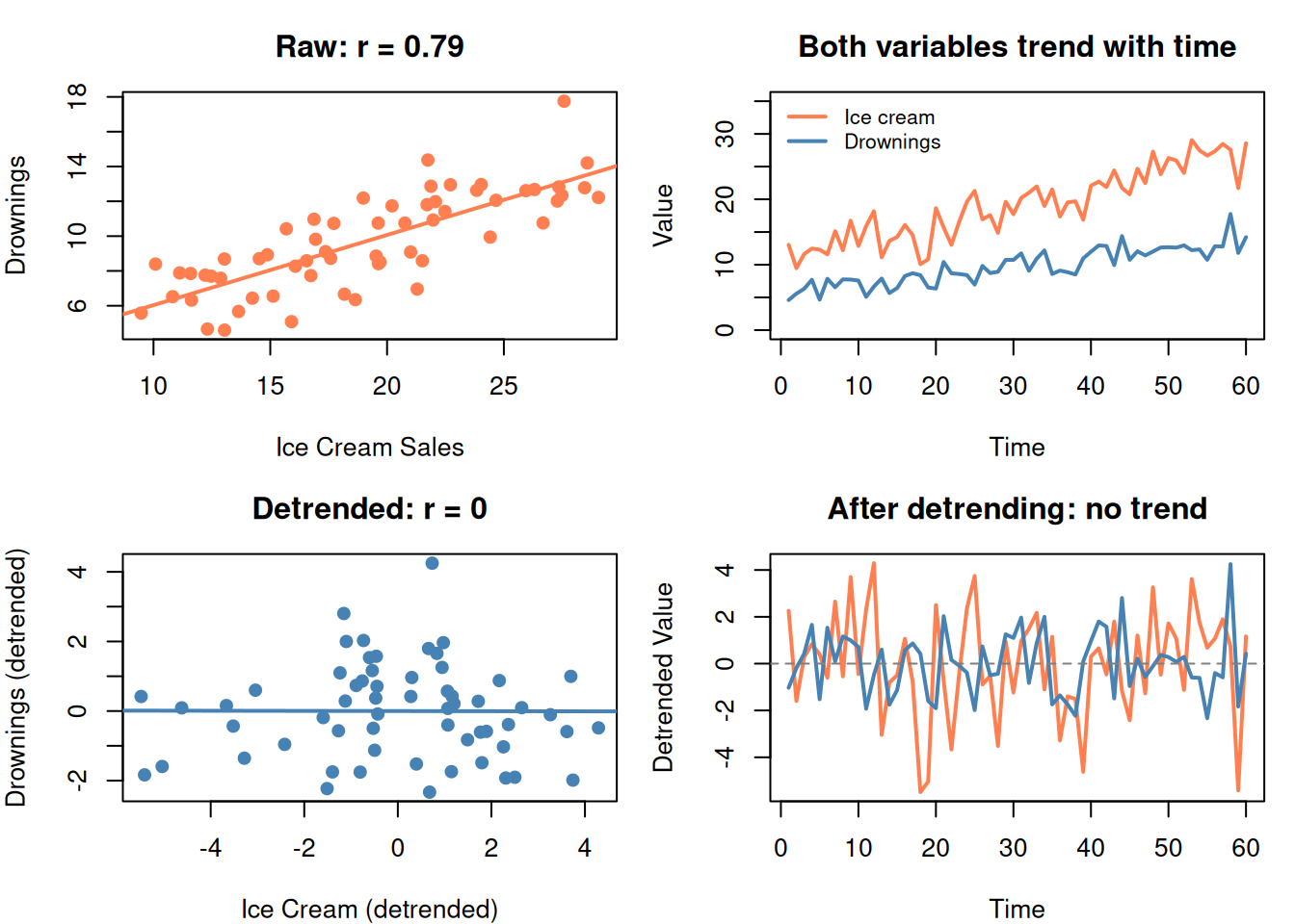
# Two UNRELATED things that both trend upward
ice_cream <- 10 + 0.3 * time_dt + rnorm(60, 0, 2)
drownings <- 5 + 0.15 * time_dt + rnorm(60, 0, 1.5)

par(mfrow = c(2, 2), mar = c(4, 4, 3, 1))

# Raw correlation (spurious)
plot(ice_cream, drownings, pch = 19, col = "coral",
  main = paste0("Raw: r = ", round(cor(ice_cream, drownings), 2)),
  xlab = "Ice Cream Sales", ylab = "Drownings")
abline(lm(drownings ~ ice_cream), col = "coral", lwd = 2)

# Both trending
plot(time_dt, ice_cream, type = "l", col = "coral", lwd = 2,
  main = "Both variables trend with time",
  xlab = "Time", ylab = "Value", ylim = c(0, 35))
lines(time_dt, drownings, col = "steelblue", lwd = 2)
legend("topleft", legend = c("Ice cream", "Drownings"), bty = "n",
  col = c("coral", "steelblue"), lwd = 2, cex = 0.8)

# Detrend
ice_dt <- residuals(lm(ice_cream ~ time_dt))
drown_dt <- residuals(lm(drownings ~ time_dt))

# Detrended correlation (real)
plot(ice_dt, drown_dt, pch = 19, col = "steelblue",
  main = paste0("Detrended: r = ", round(cor(ice_dt, drown_dt), 2)),
  xlab = "Ice Cream (detrended)", ylab = "Drownings (detrended)")
abline(lm(drown_dt ~ ice_dt), col = "steelblue", lwd = 2)

# Detrended series
plot(time_dt, ice_dt, type = "l", col = "coral", lwd = 2,
  main = "After detrending: no trend",
  xlab = "Time", ylab = "Detrended Value")
lines(time_dt, drown_dt, col = "steelblue", lwd = 2)
abline(h = 0, lty = 2, col = "gray50")

par(mfrow = c(1, 1))

Figure 10: Both variables trend upward with time → spurious correlation. Detrending reveals the truth.

After removing the time trend, the spurious correlation disappears.

11. PCA + Regression: The Full Workflow

The typical use of PCA in this guide:

1. You have many correlated predictors
2. Run PCA to get uncorrelated components
3. Use cross-validation to decide how many components to keep
4. Feed components into regression (or SVM, KNN, etc.)
5. Validate the final model on test data

# Use the 10-feature data from earlier
y_demo <- 2 * hidden1 - 1.5 * hidden2 + rnorm(n, 0, 0.5)

# Full regression (all 10 features)
fit_full <- lm(y_demo ~ features)

# PCA regression (3 components)
scores3 <- pca10$x[, 1:3]
fit_pca <- lm(y_demo ~ scores3)

cat("=== Full model (10 predictors) ===\n")

=== Full model (10 predictors) ===

cat(sprintf("  R² = %.3f\n", summary(fit_full)$r.squared))

  R² = 0.912

cat(sprintf("  Adj R² = %.3f\n\n", summary(fit_full)$adj.r.squared))

  Adj R² = 0.902

cat("=== PCA model (3 components) ===\n")

=== PCA model (3 components) ===

cat(sprintf("  R² = %.3f\n", summary(fit_pca)$r.squared))

  R² = 0.871

cat(sprintf("  Adj R² = %.3f\n", summary(fit_pca)$adj.r.squared))

  Adj R² = 0.867

cat("\n10 predictors → 3 components with similar Adj R²")

10 predictors → 3 components with similar Adj R²

cat("\nSimpler model, less overfitting risk, no multicollinearity")

Simpler model, less overfitting risk, no multicollinearity

12. Cheat Sheet: The Whole Story on One Page

PCA RECIPE
==========

1. PURPOSE: Compress many correlated features into fewer uncorrelated components

2. ALGORITHM:
   Standardize → Covariance matrix → Eigenvalues/vectors → Sort by variance

3. KEY CONCEPTS:
   Eigenvector = direction of spread (becomes a component)
   Eigenvalue = how much variance in that direction
   PC1 = most variance, PC2 = second most, etc.

4. HOW MANY COMPONENTS?
   Scree plot elbow OR cumulative variance ≥ 80-90%

5. CRITICAL TRAP:
   PCA ranks by VARIANCE in X, not by PREDICTIVE POWER for Y
   High-variance PC might be noise. Low-variance PC might be the signal.
   ALWAYS validate with cross-validation.

6. REQUIREMENTS:
   - ALWAYS standardize first (scale. = TRUE)
   - Continuous features
   - Some correlation among features (otherwise PCA can't compress)

BOX-COX RECIPE
==============

1. PURPOSE: Stabilize variance (fix heteroscedasticity)

2. FORMULA: T(y) = (y^λ - 1) / λ

3. SPECIAL CASES:
   λ = 1  → no transform     λ = 0   → log(y)
   λ = 0.5 → √y              λ = -1  → 1/y

4. HOW: R finds optimal λ automatically (boxcox function)

5. WHEN: Residual plot shows funnel shape (variance not constant)

DETRENDING
==========
Remove time trend before analyzing relationships:
  y_detrended = y - (a₀ + a₁ × time)
Prevents spurious correlations caused by shared time trends.

13. Check Your Understanding

NoteTest Yourself

Before moving on, try to answer these without scrolling up:

1. What problem does PCA solve? When would you use it?
2. What is an eigenvector in PCA terms? What does the eigenvalue tell you?
3. Why must you standardize before PCA?
4. You run PCA and keep only PC1 and PC2 (85% variance). A colleague says you’re losing important information. Could they be right? Why?
5. What does Box-Cox fix? How do you detect the problem it solves?
6. \(\lambda = 0\) in Box-Cox means you should apply which transformation?
7. You find a strong correlation between umbrella sales and car accidents. What should you do before concluding umbrellas cause accidents?
8. PCA gives you 5 components from 20 features. How do you decide which components to keep?